Probabilities in a Normal Distribution - TI-84
TLDRThis instructional video demonstrates how to calculate probabilities for normally distributed data using the TI-84 family of graphing calculators, focusing on the TI-84 Plus Color Edition. It guides viewers through finding the probability of utility bills in a city being less than $85, between $90 and $120, and greater than $130, given a mean of $110 and a standard deviation of $13. The video emphasizes the efficiency of using the calculator's normal cumulative distribution function (CDF) over traditional z-score table lookups, providing step-by-step instructions and interpretations of the results.
Takeaways
- 📚 The video provides a tutorial on how to calculate probabilities for normally distributed data using the TI-84 family of graphing calculators.
- 🖍️ The specific model used in the video is the TI-84 Plus Color Edition, but the process is applicable to other models like the TI-83 and TI-84.
- 📈 The example given involves calculating probabilities for monthly utility bills in a city, which are normally distributed with a mean of $110 and a standard deviation of $13.
- 📉 The video demonstrates how to find the probability of a utility bill being less than $85, between $90 and $120, and more than $130 without converting to z-scores first.
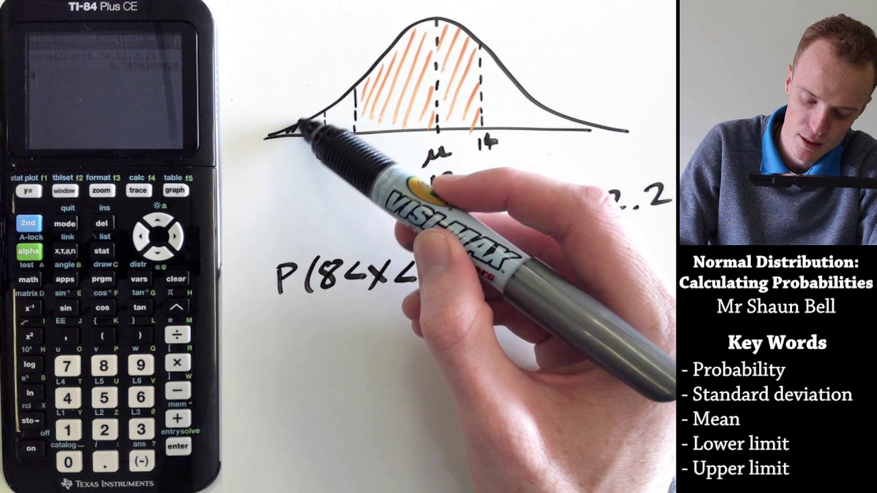
- 🎨 The importance of drawing a picture to visualize the problem and understand the areas under the normal distribution curve is highlighted.
- 📝 The script explains the parameters needed for the normal distribution: mean (μ = $110) and standard deviation (σ = $13).
- 🔢 The process of using the normal cumulative distribution function (CDF) on the calculator is detailed, including how to input values for the lower and upper limits, mean, and standard deviation.
- 🔍 The video emphasizes the use of scientific notation for entering very large or small numbers, such as negative infinity, on the calculator.
- 📊 The script illustrates how to interpret the calculator's output, providing the probability percentages for the different scenarios presented.
- 🤔 The video suggests that probabilities less than 5% are considered unusual, providing a context for understanding the results of the calculations.
- 👍 The tutorial concludes by encouraging viewers to develop an intuitive feel for what probabilities are considered unlikely through further study of statistics.
Q & A
What is the main topic of the video?
-The main topic of the video is to teach how to find probabilities for normally distributed data using the TI-84 family of graphing calculators.
Which calculator model is specifically used in the video?
-The TI-84 Plus Color Edition is specifically used in the video, but the process can also be applied to other TI-83 or TI-84 models.
What are the mean and standard deviation of the normally distributed monthly utility bills mentioned in the video?
-The mean of the monthly utility bills is $110, and the standard deviation is $13.
What are the three specific probabilities the video aims to calculate?
-The video aims to calculate the probabilities of a utility bill being less than $85, between $90 and $120, and more than $130.
Why is it suggested not to convert to z-scores first when using a graphing calculator?
-It is suggested not to convert to z-scores first because using the graphing calculator's built-in functions for normal cumulative distribution function (CDF) is much quicker and easier.
What is the normal CDF and why is it used in this context?
-The normal CDF stands for normal cumulative distribution function, which calculates the cumulative area under the normal distribution curve up to a certain point, and is used here to find probabilities without using z-tables.
How does the video demonstrate the process of finding the probability of a utility bill being less than $85?
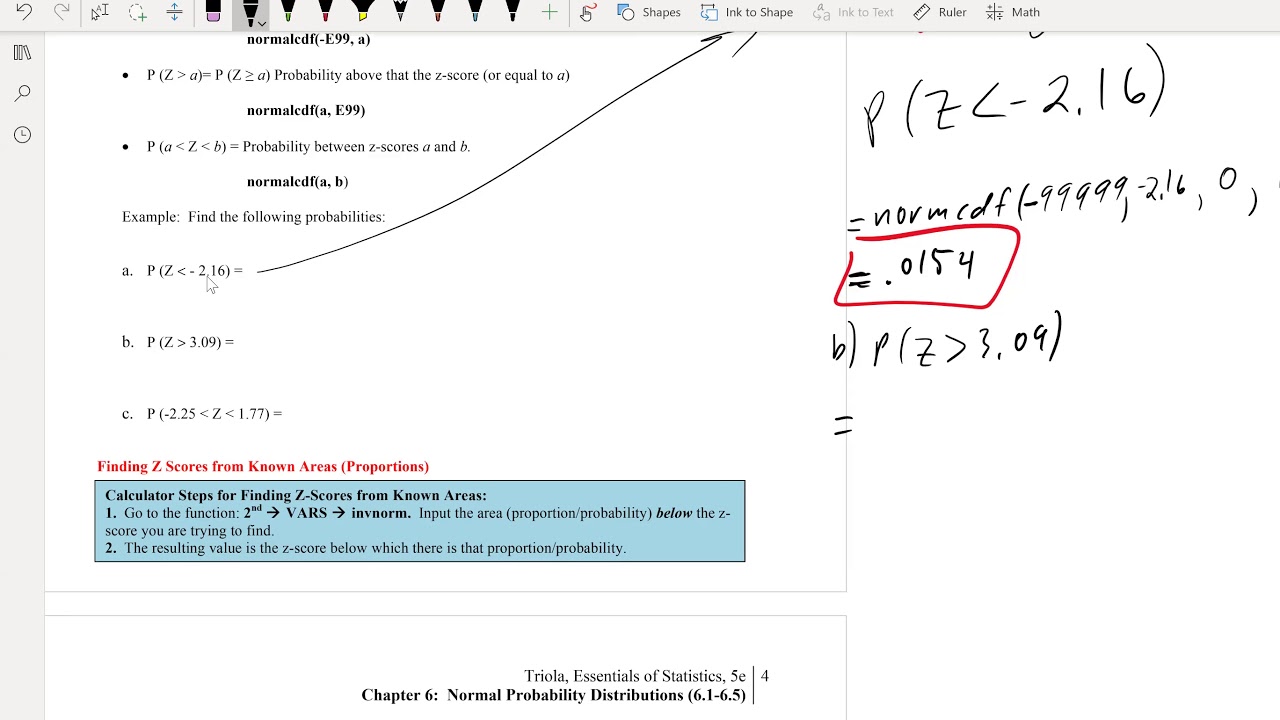
-The video demonstrates by showing how to input the values into the calculator, including using negative infinity as the lower limit, 85 as the upper limit, and the given mean and standard deviation.
What is the approximate probability of selecting a utility bill less than $85 according to the video?
-The approximate probability of selecting a utility bill less than $85 is 2.72%.
How does the video explain the probability of a bill being between $90 and $120?
-The video explains by using the normal CDF function on the calculator with 90 as the lower limit and 120 as the upper limit, and then interpreting the result as the probability.
What is the approximate probability of selecting a bill between $90 and $120 according to the video?
-The approximate probability of selecting a bill between $90 and $120 is 71.72%.
How does the video calculate the probability of a bill being more than $130?
-The video calculates this by using the normal CDF function with 130 as the lower limit and positive infinity represented by 1E99 as the upper limit, and then interpreting the result.
What is the approximate probability of selecting a bill more than $130 according to the video?
-The approximate probability of selecting a bill more than $130 is about 6%.
Outlines
📚 Introduction to Probability Calculations with TI-84
This paragraph introduces the video's purpose, which is to demonstrate how to calculate probabilities for normally distributed data using the TI-84 family of graphing calculators, specifically the TI-84 plus color edition. The example given involves calculating the probability of a utility bill in a city falling within certain ranges, based on a normal distribution with a mean of $110 and a standard deviation of $13. The video emphasizes the efficiency of using a graphing calculator over traditional z-score methods and begins by addressing the probability of a bill being less than $85, including a detailed explanation of setting up the normal distribution curve and identifying the area of interest.
🔍 Calculating the Probability of a Low Utility Bill
In this paragraph, the focus is on calculating the probability of a utility bill being less than $85 using the TI-84 calculator. The process involves using the normal cumulative distribution function (CDF) to find the area under the curve to the left of $85. The video provides a step-by-step guide on entering the necessary values into the calculator, including using negative infinity as the lower limit and 85 as the upper limit, with a mean of $110 and a standard deviation of $13. The result is interpreted to mean that there is a 2.72% chance of a bill being less than $85, which is considered unusual based on the context provided.
📉 Probability of a Utility Bill within a Specific Range
The third paragraph explains how to find the probability that a utility bill falls between $90 and $120. The video describes the process of using the normal CDF again, this time with 90 as the lower limit and 120 as the upper limit, while keeping the mean and standard deviation the same. The explanation includes a brief sketch to visualize the area under the curve that corresponds to this range. The calculator input is demonstrated, and the result shows approximately a 71.72% chance of a bill being within this range, which is a common occurrence.
📈 Probability of an Excessively High Utility Bill
The final paragraph of the script discusses calculating the probability of a utility bill exceeding $130. The video illustrates the process by using the normal CDF with 130 as the lower limit and positive infinity represented by 1E99 as the upper limit. The calculation is shown with the same mean and standard deviation as before. The result indicates a roughly 6% chance of a bill being more than $130, which is on the borderline of being considered unusual. The video concludes by emphasizing the importance of understanding the distribution and the calculator's output to avoid mistakes and gain a better intuitive feel for what probabilities are considered unlikely.
Mindmap
Keywords
💡Normal Distribution
💡TI-84 Calculator
💡Mean
💡Standard Deviation
💡Probability
💡Cumulative Distribution Function (CDF)
💡Z-Score
💡Graphical Representation
💡Interpretation
💡Unusual Events
💡Scientific Notation
Highlights
Introduction to finding probabilities for normally distributed data using TI-84 calculators.
Demonstration using the TI-84 Plus Color Edition, with applicability to other TI-83/84 models.
Explanation of a normally distributed monthly utility bill scenario with a mean of $110 and standard deviation of $13.
Three probability scenarios: less than $85, between $90 and $120, and more than $130.
Advantage of using a graphing calculator over traditional z-score tables for quicker calculations.
Visual representation of the normal distribution with mean and standard deviation.
Graphical depiction of one, two, and three standard deviations from the mean.
Procedure to calculate the probability of a utility bill being less than $85.
Using the normal cumulative distribution function (CDF) on the calculator.
Entering negative infinity as the lower limit and 85 as the upper limit for the calculation.
Explanation of how to input values into the TI-84 calculator for the normal CDF function.
Interpretation of the result showing a 2.72% probability of a bill being less than $85.
Calculating the probability of a bill being between $90 and $120.
Graphical representation of the area between $90 and $120 on the normal distribution curve.
Entering the values 90 and 120 into the calculator for the specified range probability.
Result interpretation indicating a 71.72% chance of a bill falling between $90 and $120.
Calculating the probability of a bill exceeding $130.
Using positive infinity as the upper limit in the calculator for probabilities greater than a value.
Final result interpretation with a 6% chance of a bill being over $130, considered unusual.
Conclusion emphasizing the importance of understanding normal distribution for statistical analysis.
Transcripts

5.0 / 5 (0 votes)
Thanks for rating: