Linear Demand Equations - part 2 (NEW 2016!)

Jason Welker

5 Sept 201605:50

EducationalLearning

32 Likes 10 Comments

TLDRIn this lesson, the instructor explores the application of a linear demand equation derived from a demand schedule or curve. They demonstrate how to calculate the quantity demanded at various prices, including those not directly observable on the demand curve. The instructor also explains how to determine the price intercept, where the demand curve begins, by setting the quantity demanded to zero and solving for the price. The session concludes with a preview of upcoming topics, such as factors that can shift the demand curve and affect the equation's variables.

Takeaways

📚 The lesson focuses on understanding how to derive a linear demand equation from data and how to calculate quantities demanded at different prices.
📉 The 'a' and 'b' variables in the demand equation represent the intercept and slope of the demand curve, respectively, and are crucial for calculating demand at various prices.
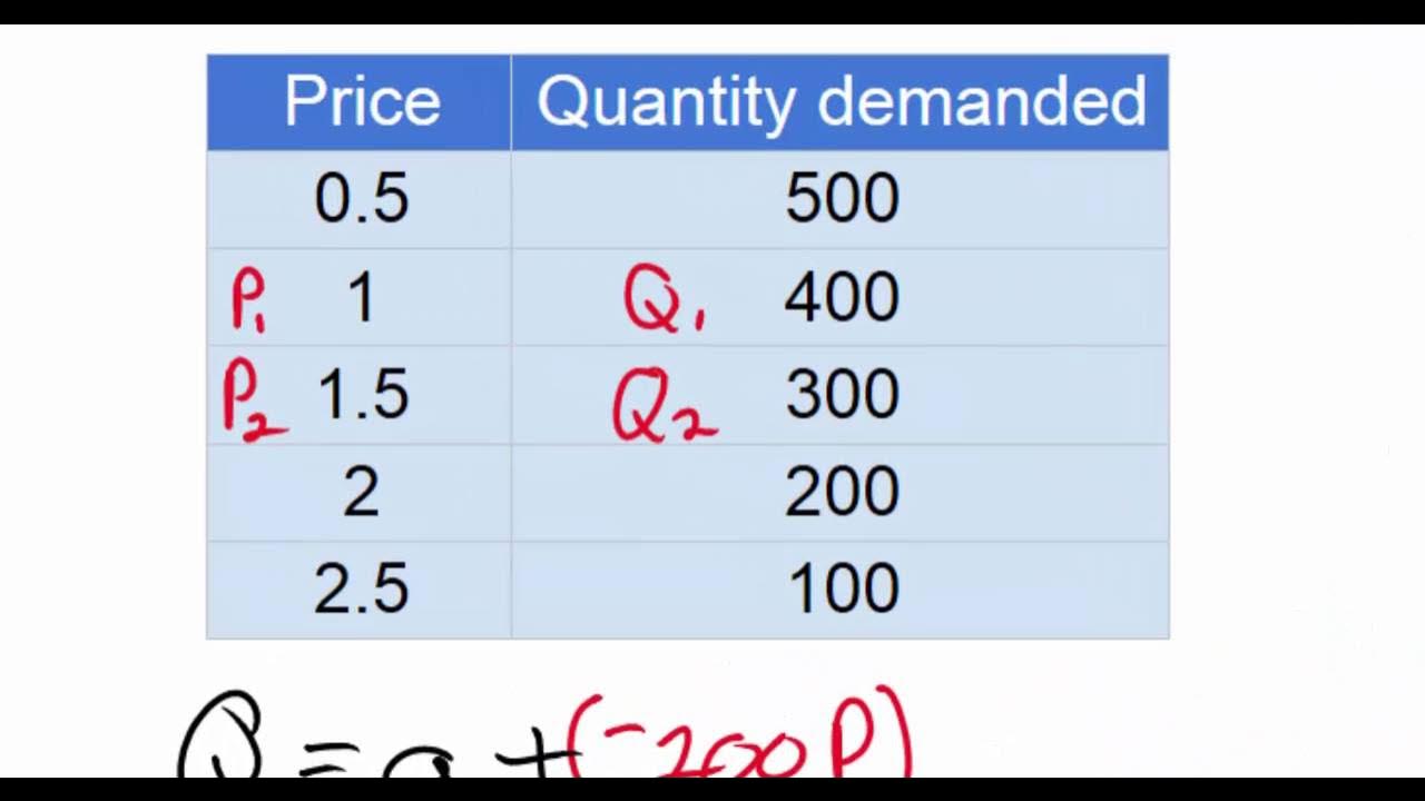
🍬 The example given is a demand equation for candy among 68 students, with the equation Qd = 600 - 200P, where Qd is the quantity demanded and P is the price.
🔢 The script demonstrates how to use the demand equation to find the exact quantity demanded at a price not directly observable on the demand curve or schedule, such as at $1.72.
🧮 Through the example, it is shown that at a price of $1.72, the quantity demanded would be 256 units of candy, calculated by substituting the price into the demand equation.
📉 The P intercept, or price intercept, is the point where the demand curve intersects the vertical axis, indicating the price at which quantity demanded equals zero.
💡 The P intercept can be calculated by setting the quantity demanded to zero in the demand equation and solving for the price, which in the example is $3.
🔑 The demand equation allows for precise determination of quantity demanded at any price, between the Q intercept and the P intercept.
🛑 The lesson concludes with a promise to discuss factors that can shift the demand curve in the next lesson, affecting both the 'a' and 'b' variables in the demand equation.
🔄 The shift in the demand curve can be due to changes in consumer preferences, income, price of related goods, and other market conditions.

Q & A

What is the purpose of deriving a linear demand equation?
-The purpose of deriving a linear demand equation is to represent the relationship between the quantity of a product demanded and its price, making it possible to calculate the quantity demanded at different price points.
How can you calculate the 'a' and 'b' variables in a linear demand equation?
-The 'a' and 'b' variables in a linear demand equation can be calculated using data from a demand schedule or a demand curve. The 'a' variable is the intercept, and the 'b' variable is the slope, which is the price coefficient.
What is the formula for the linear demand equation mentioned in the script?
-The formula for the linear demand equation mentioned in the script is Quantity Demanded (QD) = a - b * Price (P), where 'a' is the intercept and 'b' is the price coefficient.
How can you determine the quantity demanded at a specific price using the demand equation?
-To determine the quantity demanded at a specific price, you substitute the price into the demand equation and solve for the quantity demanded (QD).

Outlines

00:00

📚 Introduction to Linear Demand Equations

This paragraph introduces the concept of linear demand equations and how they are derived from demand schedules or curves. The speaker demonstrates the calculation of the 'a' and 'B' variables in the equation and uses the equation to determine the quantity of candy demanded at a specific price. The paragraph also touches on the potential changes in the demand equation that could cause shifts in the demand curve, including alterations to the 'a' variable and the price coefficient 'B'. The speaker provides a practical example of calculating the quantity demanded at a price not directly observable from the demand schedule or curve, using the derived demand equation to find the exact quantity demanded at $1.72.

05:02

📉 Calculating Price Intercepts and Demand Curve Shifts

The second paragraph delves into the calculation of the price intercept (P intercept) of the demand curve, which is the point where the quantity demanded equals zero. The speaker explains that this can be easily identified in a linear demand equation, as demonstrated with an example where the P intercept is found to be $3. The paragraph also discusses the method for determining the P intercept when it is not immediately clear from the demand curve, which involves setting the quantity demanded to zero and solving for the price. The speaker concludes by mentioning that the next lesson will cover factors that can shift the demand curve, affecting both the 'a' variable and the 'B' variable in the demand equation.

Mindmap

Keywords

💡Linear Demand

Linear demand refers to a type of demand curve that has a straight line representation, where the quantity demanded of a good is inversely proportional to its price, assuming all other factors remain constant. In the video, the concept is central as the instructor explains how to derive and use a linear demand equation to calculate quantities demanded at different prices.

💡Demand Equation

A demand equation is a mathematical formula that represents the relationship between the quantity demanded of a product and its price. In the script, the demand equation is derived as 'quantity demanded = 600 - 200 * price', which is used to calculate how many units of candy would be demanded at various price points.

💡Price

Price is the amount of money required to purchase a good or service. The video script discusses how different prices affect the quantity demanded, using the example of candy where at $1.72, the quantity demanded is calculated to be 256 units.

💡Quantity Demanded

Quantity demanded is the amount of a product that consumers are willing and able to purchase at a given price. The video demonstrates calculating this for various prices, such as 300 units at $150 and 256 units at $1.72.

💡Demand Schedule

A demand schedule lists the quantities of a product that consumers are willing to buy at various prices. The script mentions using a demand schedule to derive the linear demand equation.

💡Demand Curve

A demand curve is a graphical representation of the demand schedule, showing the relationship between the price of a good and the quantity demanded. The video script uses the demand curve to illustrate quantities demanded at specific prices and to identify the price and quantity intercepts.

💡A Variable

In the context of the demand equation, the 'A variable' represents the y-intercept, which is the quantity demanded when the price is zero. In the script, the 'A variable' is 600, indicating that 600 units of candy would be demanded if the price were free.

💡B Variable

The 'B variable' in the demand equation is the slope of the demand curve, indicating how sensitive the quantity demanded is to price changes. In the video, the 'B variable' is -200, meaning for every unit increase in price, the quantity demanded decreases by 200 units.

💡Price Intercept

The price intercept, or P intercept, is the point where the demand curve intersects the price axis, indicating the price at which the quantity demanded is zero. The script explains how to calculate this intercept using the demand equation, which in the example is $3.

💡Shift in Demand Curve

A shift in the demand curve refers to a change in consumer preferences or other factors that cause the entire demand curve to move either to the right (increase in demand) or to the left (decrease in demand). The script mentions that changes in the 'A' and/or 'B' variables can cause such shifts.

💡Factors Affecting Demand

Factors affecting demand are variables that influence the quantity of a product that consumers are willing to buy. The script suggests that changes in these factors can alter the 'A' and 'B' variables in the demand equation, leading to shifts in the demand curve.

Highlights

Introduction to deriving a linear demand equation from a demand schedule or curve.

Explanation of calculating the 'a' and 'b' variables in the demand equation.

Demonstration of using the demand equation to calculate quantities demanded at different prices.

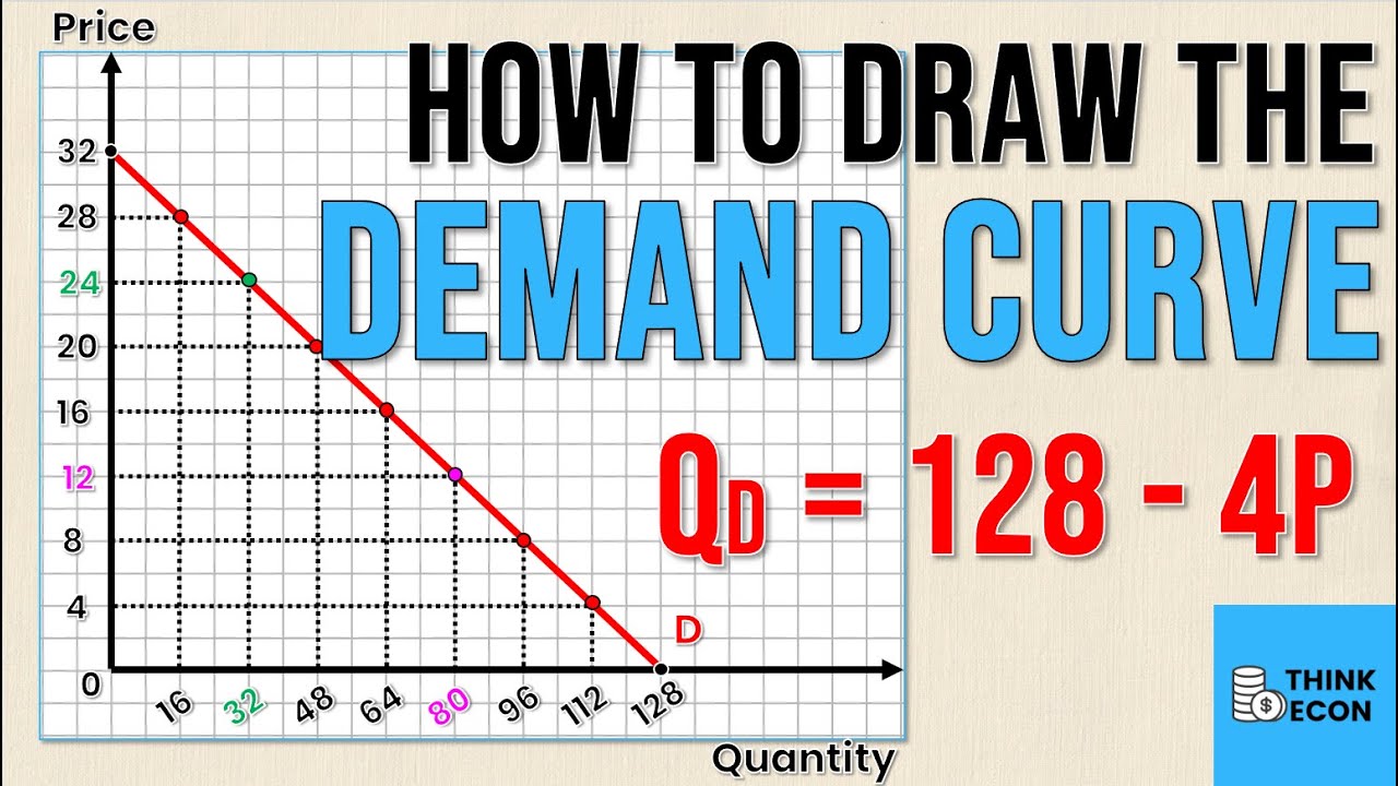
Visual representation of the demand curve and how to read quantities at specific prices.

Method to determine the exact quantity demanded at a price not directly observable on the demand curve.

Calculation of the quantity demanded at a specific price of $1.72 using the demand equation.

Explanation of the demand equation's utility in determining quantities at any price point.

Introduction to the concept of the price intercept (P intercept) of demand.

How to calculate the price intercept when the demand curve does not intersect the P-axis at an obvious point.

Demonstration of solving for the price intercept by setting the quantity demanded to zero.

Verification of the P intercept for the given demand equation being $3.

Discussion on the practicality of the method for determining the P intercept in non-obvious cases.

Teaser for the next lesson focusing on factors that can shift the demand curve.

Anticipation of discussing changes in the 'a' variable and 'b' variable in the demand equation.

Emphasis on the importance of understanding the factors that influence demand shifts.

Conclusion of the lesson with a summary of the key points covered.

Transcripts

Browse More Related Video

Linear Demand Equations - part 1

Linear Demand Equations - part 1(NEW 2016)

How to Draw the DEMAND CURVE (Using the DEMAND EQUATION) | Think Econ

Understanding the Demand Curve: Shifts and Consumer Surplus

Math 11 - Section 3.7

Managerial Economics 2.5: More Elasticity