Linear Demand Equations - part 1(NEW 2016)

Jason Welker

5 Sept 201610:28

EducationalLearning

32 Likes 10 Comments

TLDRIn this lesson, the speaker explains how to derive a demand equation from a demand schedule or curve. Using an example of candy demand from a class survey, the lesson highlights the inverse relationship between price and quantity demanded. The process involves calculating the 'B' variable (inverse of slope) and the 'A' variable (quantity demanded at zero price) to formulate the equation Q = A + BP. This method reverses the traditional Y = MX + B formula by treating price as the independent variable and quantity as the dependent variable, making it easier to understand linear demand relationships.

Takeaways

📚 The lesson aims to show how to derive a demand equation using a demand schedule or curve.
📈 The law of demand is demonstrated with a graph showing higher quantity demanded at lower prices.
🔄 The traditional y = mx + b equation is flipped for demand, making quantity (Q) the dependent variable on price (P).
📉 The demand equation is represented as Q = a + bP, where 'a' is the quantity demanded when price is zero and 'b' is the inverse of the slope.
⚖️ The 'b' variable is calculated by finding the change in quantity over the change in price from the demand schedule.
🔢 The 'a' variable is determined by plugging a known quantity and price into the demand equation and solving for 'a'.
📉 'B' is always negative, reflecting the inverse relationship between price and quantity demanded.
📋 To find the demand equation, first calculate the 'b' variable using two points from the demand schedule, then find 'a' by using a point on the demand curve.
📊 The derived demand equation can be used to understand how quantity demanded changes with price variations.
🔍 Future lessons will discuss factors that can change 'a' or 'b' and their effects on the demand curve's shape, position, or slope.
🎓 The lesson concludes by emphasizing the importance of understanding the steps to determine the linear demand curve equation.

Q & A

What is the main topic of the lesson in the provided transcript?
-The main topic of the lesson is deriving a demand equation using data from a demand schedule or a demand curve.
What is the law of demand as illustrated in the script?
-The law of demand, as illustrated, states that at lower prices, there is a higher quantity of a good demanded, and at higher prices, there is a lower quantity demanded.
Why can't the traditional linear equation y = mx + b be used to represent demand?
-The traditional linear equation y = mx + b cannot be used for demand because in demand, the quantity demanded (Q) is the dependent variable, which depends on the price (P), not the other way around.
What is the correct equation format to represent demand for a good?
-The correct equation format to represent demand for a good is Q = a + bP, where Q is the quantity demanded, a is the Q intercept, b is the inverse of the slope, and P is the price.

Outlines

00:00

📚 Deriving a Demand Equation from a Linear Relationship

This paragraph introduces the process of deriving a demand equation using a linear demand schedule or curve. It begins with a real-world example of survey data on candy demand at various prices, illustrating the law of demand where higher quantities are demanded at lower prices. The speaker explains the need to invert the traditional linear equation (y = mx + b) to fit the demand relationship where quantity demanded (Q) is the dependent variable and price is the independent variable. The demand equation is presented as Q = a + bP, where 'a' is the quantity demanded when the price is zero (autonomous demand), and 'b' is the inverse of the slope, indicating the change in quantity for a given change in price.

05:03

🔍 Calculating the Demand Equation Variables

The second paragraph delves into calculating the variables 'a' and 'b' for the demand equation using data from a demand schedule. The speaker demonstrates how to find 'b' by using the change in quantity (Q2 - Q1) divided by the change in price (P2 - P1), resulting in a negative value due to the inverse relationship between price and quantity demanded. The 'a' variable is determined by plugging in a known quantity and price into the demand equation and solving for 'a'. The example given uses specific values from the demand schedule to calculate both variables, ultimately providing the complete demand equation for candy. The paragraph concludes with an explanation of the 'b' variable as the inverse of the slope, emphasizing the relationship between price changes and quantity demanded.

10:04

📈 Understanding the Factors Influencing Demand Equation Variables

The final paragraph hints at future lessons that will explore the factors affecting the 'a' and 'b' variables in the demand equation, and how these changes can influence the demand curve's shape, position, or slope. The speaker emphasizes the importance of understanding these factors to analyze market dynamics effectively. This sets the stage for a deeper dive into the complexities of demand and its determinants in subsequent educational content.

Mindmap

Keywords

💡Demand Equation

A demand equation is a mathematical representation that describes the relationship between the quantity of a good that consumers are willing to purchase and its price. In the video, the instructor illustrates how to derive this equation from a demand schedule or a demand curve, which is essential for understanding consumer behavior and market dynamics.

💡Demand Schedule

A demand schedule is a table that lists the quantities of a product that consumers are willing to buy at various prices over a certain period. It serves as a foundational data set for deriving the demand equation, as demonstrated in the script where the instructor uses survey data to create a demand schedule for candy at different prices.

💡Demand Curve

A demand curve is a graphical representation showing the relationship between the quantity demanded of a good and its price. In the video, the instructor discusses how to derive a demand equation from a demand curve, which typically has a downward slope indicating the law of demand—that as price decreases, quantity demanded increases.

💡Law of Demand

The law of demand states that, all else being equal, as the price of a good increases, the quantity demanded decreases; conversely, the lower the price, the greater the quantity demanded. The video script provides a clear visual example of this law through the demand curve for candy.

💡Linear Relationship

A linear relationship implies a direct proportionality between two variables, which can be represented by a straight line on a graph. The video script simplifies the actual data to a linear relationship to demonstrate deriving a demand equation, even though real-world data might not be perfectly linear.

💡Dependent Variable

In the context of the demand equation, the dependent variable is the quantity demanded, which varies in response to changes in the price. The video explains that in the standard linear equation (y = mx + b), y is the dependent variable, but for demand, the quantity demanded (Q) is dependent on the price (P).

💡Slope

Slope is a measure of the steepness of a line, indicating the rate of change of the dependent variable with respect to the independent variable. In the video, the instructor discusses how the slope is represented differently in a demand equation compared to the standard linear equation, as it is the inverse of the slope (run over rise).

💡Q Intercept

The Q intercept, also known as the quantity intercept, is the point where the demand curve crosses the quantity axis (Q = 0). It represents the quantity demanded when the price is zero. The video script explains how to calculate this intercept as part of deriving the demand equation.

💡Autonomous Demand

Autonomous demand refers to the quantity of a good that consumers would demand even if the price were zero. In the video, the instructor uses the term to describe the Q intercept, which is the quantity demanded if the good were free.

💡Inverse Relationship

An inverse relationship is a type of relationship between two variables where an increase in one variable results in a decrease in the other. The video script explains that there is an inverse relationship between price and quantity demanded, which is why the B variable in the demand equation is negative.

💡Calculating the B Variable

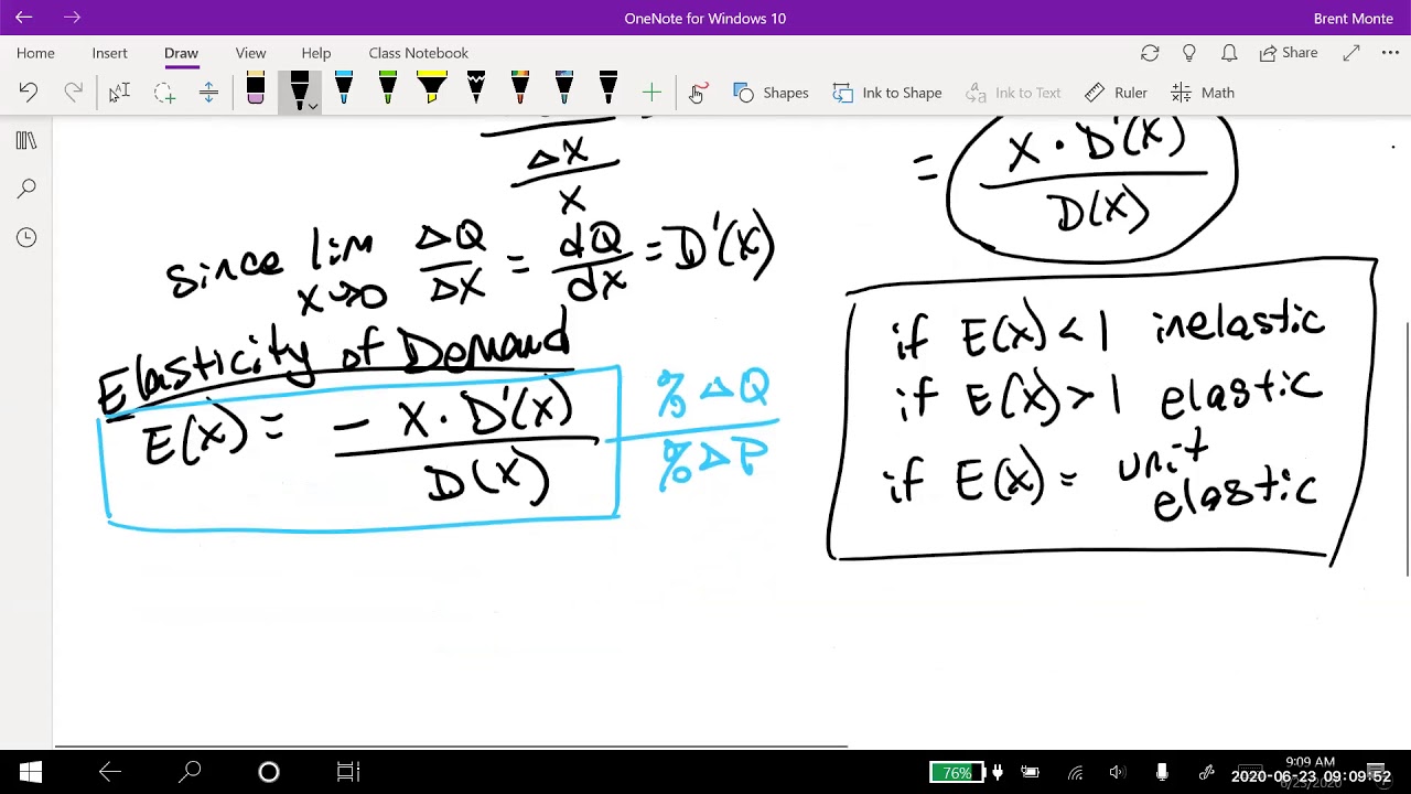
The B variable in the demand equation is calculated by finding the change in quantity divided by the change in price between two points on the demand curve. The video provides a step-by-step example of how to calculate this using data from the demand schedule.

💡Price Elasticity of Demand

Price elasticity of demand measures the responsiveness of the quantity demanded to a change in price. While not explicitly mentioned in the script, understanding the B variable as the inverse of the slope is crucial for calculating price elasticity, which is a fundamental concept in economics related to the demand equation.

Highlights

Introduction to deriving a demand equation using data from a demand schedule or demand curve.

Recap of the law of demand: Lower prices lead to higher quantity demanded.

Explanation of flipping the typical linear equation to fit the demand model.

Introduction of the demand equation: Q = a + b * P, where Q is the quantity demanded and P is the price.

Clarification that in the demand equation, quantity demanded is the dependent variable and price is the independent variable.

Explanation of the variables in the demand equation: 'a' represents the Q intercept (quantity demanded when price is zero) and 'b' represents the inverse of the slope.

Detailed process of calculating the 'b' variable using two sets of quantities and prices from the demand schedule.

Example calculation of the 'b' variable resulting in a value of -200.

Explanation that the 'b' variable will always be negative due to the inverse relationship between price and quantity demanded.

Method to calculate the 'a' variable using a chosen point from the demand schedule.

Example calculation showing the 'a' variable as 600.

Discussion on the interpretation of the complete demand equation: Q = 600 - 200 * P.

Reiteration of how the 'b' variable represents the change in quantity for a given change in price.

Summary of the steps to find a demand equation: First find the 'b' variable, then find the 'a' variable.

Mention of future lessons covering factors that can cause changes in the 'a' and 'b' variables, affecting the demand curve.

Transcripts

Browse More Related Video

Linear Demand Equations - part 1

Linear Demand Equations - part 2 (NEW 2016!)

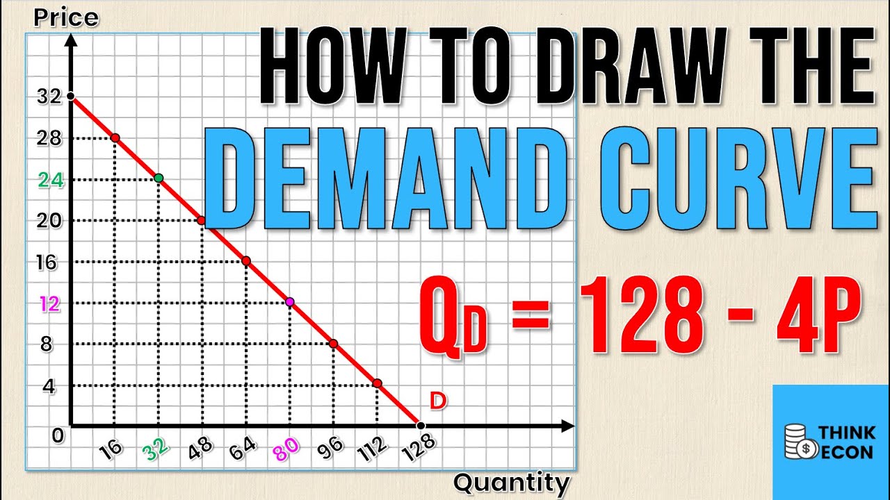
How to Draw the DEMAND CURVE (Using the DEMAND EQUATION) | Think Econ

Math 11 - Section 3.7

Elasticity Resulting From Infinite Change In Quantity Demanded [Express Revenue As A Function Of P]

Understanding the Demand Curve: Shifts and Consumer Surplus