Linear Demand Equations - part 1
TLDRThis video lesson delves into the linear demand equation, exploring its variables and their impact on the quantity demanded. It uses the example of pizza to demonstrate how demand changes with price, illustrating the inverse relationship. The lesson constructs a demand schedule and curve, highlighting the autonomous demand level and the slope's role in price sensitivity. It effectively reinforces the law of demand, showing how quantity demanded decreases as price increases.
Takeaways
- 📚 The video lesson focuses on understanding a linear demand equation for a good, specifically pizza in this case.
- 🔢 QD represents the quantity demanded for a good, which is influenced by various variables, including price.
- 🏷️ The 'a' variable in the demand equation is the autonomous level of demand, indicating the quantity demanded when the price is zero.
- ➖ The 'b' variable is crucial, showing the inverse relationship between price and quantity demanded; it is negative.
- ⚖️ For every unit increase in price, the quantity demanded decreases by the value of 'b', demonstrating the law of demand.
- 📉 The demand equation provided is QD = 800 - 60P, where 800 is the quantity demanded when price is zero, and 60 is the change in quantity for each price change.
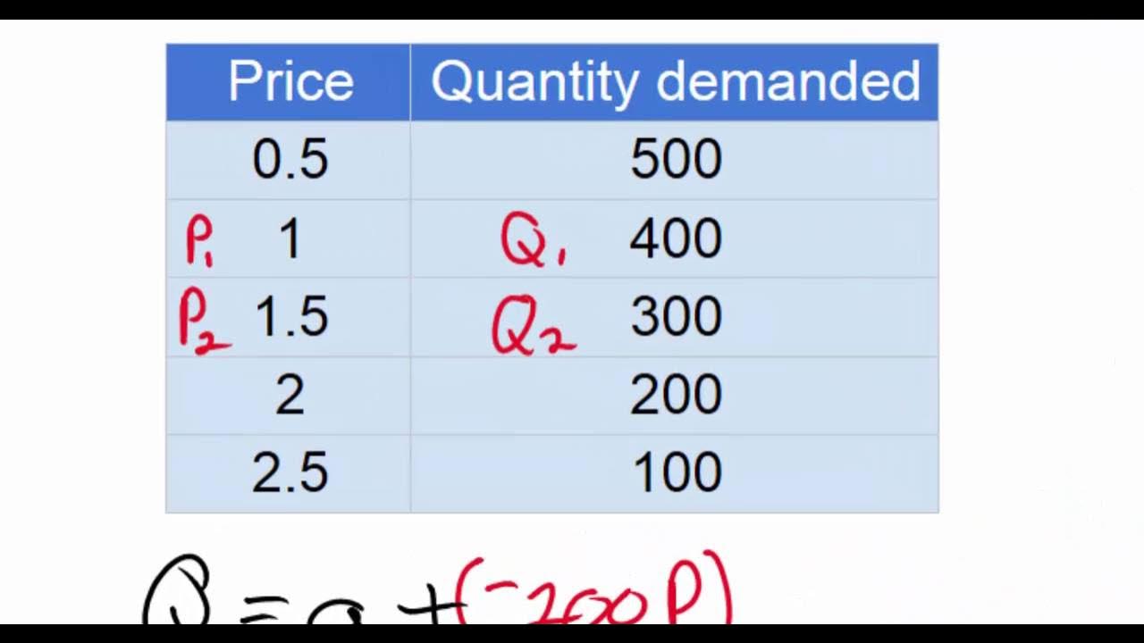
- 📈 A demand schedule is created using the demand equation, plotting quantities demanded at various prices, showing a decrease as price increases.
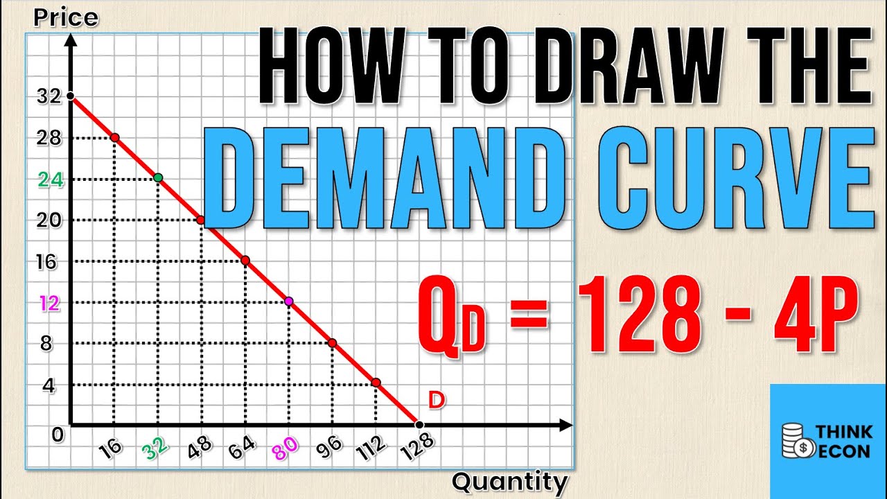
- 📊 The demand curve is plotted using at least two points from the demand schedule, illustrating the linear relationship between price and quantity demanded.
- 📍 The Q intercept (a) on the demand curve shows the quantity demanded at a price of zero, which is 800 pizzas in this example.
- 📉 As price increases, the quantity demanded decreases in increments of 120 pizzas, reflecting the -60 b variable in the demand equation.
- 📋 The lesson concludes by reinforcing the understanding of the 'a' and 'b' variables in the demand equation and their impact on the demand curve.
Q & A
What is the focus of the video lesson?
-The video lesson focuses on a linear demand equation, analyzing its variables, and using it to derive a demand schedule and a demand curve for pizza.
What does QD represent in the context of the video?
-QD represents the quantity demanded for a good, which is dependent on several variables in the linear demand equation.
What is the 'a' variable in the demand equation?
-The 'a' variable is the autonomous level of demand or the quantity intercept, indicating the quantity of the good that will be demanded when the price is zero.
What is the 'b' variable in the demand equation?
-The 'b' variable represents the slope of the demand curve, showing the rate at which quantity demanded changes in response to a change in price.
Outlines
📚 Introduction to Linear Demand Equations
This paragraph introduces the concept of a linear demand equation, focusing on the variables involved. It starts with QD, the quantity demanded, which depends on several factors. The 'a' variable represents the autonomous level of demand or the quantity demanded when the price is zero. The 'B' variable indicates the change in demand as the price changes, with a negative sign signifying an inverse relationship between price and quantity demanded. An example demand equation for pizza is given, illustrating how to derive a demand schedule and curve. The paragraph explains how the demand schedule is created by plotting quantities demanded at various prices, showing the decrease in demand as price increases, in line with the law of demand.
📈 Plotting the Demand Curve for Pizza
The second paragraph delves into the process of plotting a demand curve using the data from the demand schedule. It emphasizes the importance of the 'a' variable as the quantity intercept, showing the quantity demanded when the price is zero. The 'B' variable is likened to the slope in algebra, indicating the change in quantity for every change in price. The paragraph concludes by plotting two points on the demand graph: one where the price is zero and the quantity demanded is 800 pizzas, and another at a price of $10 with a quantity demanded of 200 pizzas. Connecting these points visually represents the demand curve for pizza, demonstrating the inverse relationship between price and quantity demanded.
Mindmap
Keywords
💡Linear Demand Equation
💡Quantity Demanded (QD)
💡Autonomous Level of Demand
💡Price
💡Inverse Relationship
💡Demand Schedule
💡Law of Demand
💡Demand Curve
💡Slope
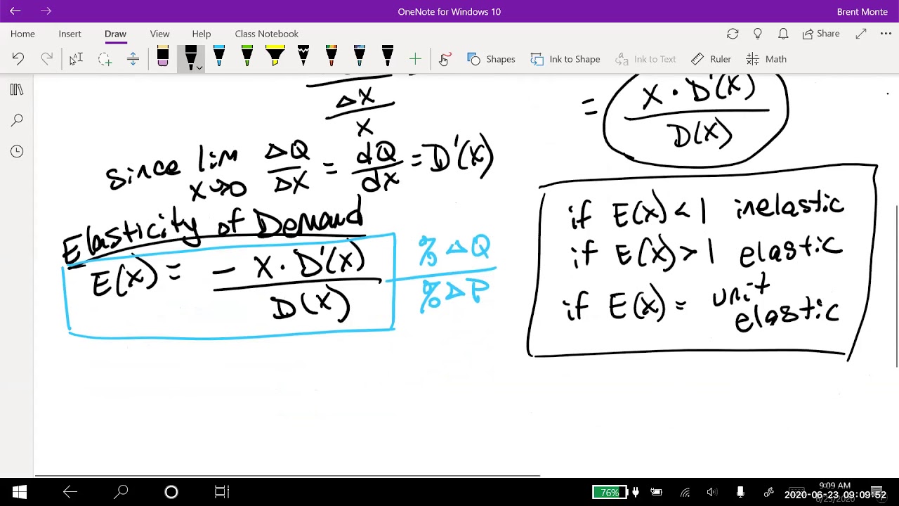
💡Price Elasticity of Demand
💡Q Intercept
Highlights
Introduction to a linear demand equation in the context of economics.
Explanation of the quantity demanded (QD) and its dependence on various factors.
Definition of the 'a' variable as the autonomous level of demand or the quantity intercept.
Clarification that 'a' represents the quantity demanded when the price is zero.
Introduction of the 'B' variable indicating the change in demand relative to price changes.
Emphasis on the negative sign of 'B' reflecting the inverse relationship between price and quantity demanded.
Presentation of the general linear demand equation: QD = a - BP.
Example given using the demand for pizza with a specific demand equation.
Creation of a demand schedule plotting quantities demanded at various prices.
Demonstration of how the quantity demanded decreases as price increases, following the law of demand.
Calculation of the new quantity demanded as price changes, using the B variable.
Description of the process to plot a demand curve using data from the demand schedule.
Identification of key points for the demand curve from the demand schedule.
Graphical representation of the demand curve for pizza with the equation QD = 800 - 60P.
Explanation of the 'a' variable as the quantity demanded at a price of zero.
Discussion on the 'B' variable's role in indicating the change in quantity for every price change.
Conclusion summarizing the variables in a demand equation.
Transcripts


5.0 / 5 (0 votes)
Thanks for rating: