How to Draw the DEMAND CURVE (Using the DEMAND EQUATION) | Think Econ
TLDRThis educational video teaches viewers how to graphically represent a demand curve using a given demand equation. Starting with graph paper and labeling axes for price and quantity, the presenter uses the linear demand equation Q = 128 - 4P to find intercepts and plot points. They demonstrate calculating the quantity and price intercepts, and how to determine corresponding Q and P values for any given price or quantity. The video encourages further exploration by suggesting the creation of a demand schedule for a comprehensive understanding of the demand curve.
Takeaways
- 📚 The video is a tutorial on how to draw a demand curve using a given demand equation.
- 📈 The demand equation provided in the video is Q = 128 - 4P, indicating a linear demand curve.
- 📊 To begin, a graph is set up with axes labeled for price and quantity.
- 🔍 The demand curve is identified as linear by its resemblance to the general form of a line, Y = mX + b.
- ✏️ The video demonstrates how to find the quantity intercept (Q intercept) by setting the price (P) to zero and solving for Q.
- 📐 Similarly, the price intercept is found by setting the quantity (Q) to zero and solving for P.
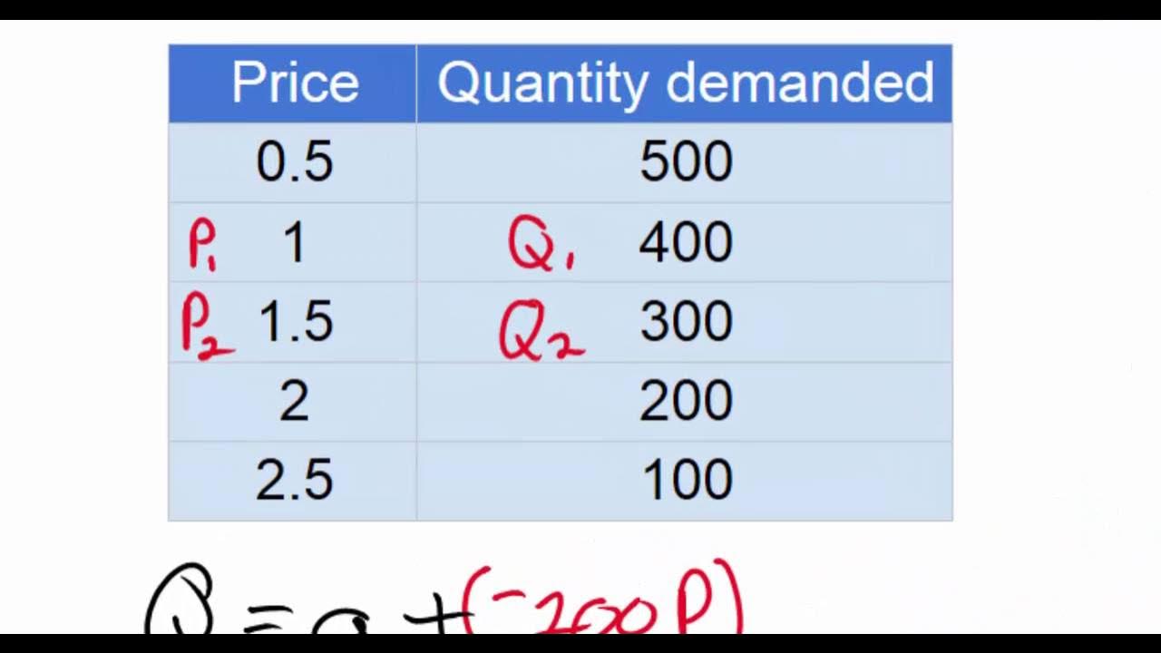
- 📝 The Q intercept is calculated to be 128, and the P intercept is 32, which are then plotted on the graph.
- 📌 Some educators may require additional points on the graph for a complete representation of the demand curve.
- 🔢 The video shows how to find corresponding Q and P values for any given price or quantity within the curve's range.
- 📋 It's suggested to create a table of values or a demand schedule for a comprehensive view of the demand curve.
- 🌐 The video emphasizes that there are infinite points between the intercepts that can be calculated using the demand equation.
- 👍 The video concludes by encouraging viewers to like, subscribe, and comment for more economic topics.
Q & A
What is the main topic of the video?
-The main topic of the video is teaching viewers how to draw a demand curve given a demand equation.
What tools are needed to start drawing the demand curve according to the video?
-To start drawing the demand curve, one needs graph paper and a demand equation.
What is the general form of a linear equation mentioned in the video?
-The general form of a linear equation mentioned in the video is Y equals mX plus b.
How does the video determine the type of demand curve?
-The video determines the type of demand curve by recognizing the demand equation's form, identifying it as linear due to its resemblance to the general form of a line.
What are the intercepts of the demand curve discussed in the video?
-The intercepts discussed in the video are the price intercept and the quantity intercept, also known as the Y and X-intercepts.
How is the quantity intercept (Q intercept) calculated in the video?
-The quantity intercept is calculated by setting the price (P) to zero in the demand equation and solving for Q, which results in Qd = 128.
What is the price intercept (P intercept) found in the video?
-The price intercept is found by setting the quantity (Q) to zero in the demand equation, resulting in P = 32.
Why might a teacher ask for multiple points on the demand curve?
-A teacher might ask for multiple points on the demand curve to provide a more detailed and accurate representation of the demand equation.
How does the video demonstrate finding a corresponding quantity for a given price?
-The video demonstrates finding a corresponding quantity for a given price by substituting the price into the demand equation and solving for Q, as shown with a price of $24.
How does the video show finding the corresponding price for a given quantity?
-The video shows finding the corresponding price for a given quantity by substituting the quantity into the demand equation, rearranging to solve for P, as demonstrated with a quantity of 80.
What additional tool is suggested for better understanding of the demand curve in the video?
-The video suggests creating a table of values or a demand schedule as an additional tool for better understanding of the demand curve.
What is the maximum price and quantity indicated by the intercepts in the video?
-The maximum price indicated by the intercepts is $32, and the maximum quantity is 128.
How does the video suggest finding an infinite number of values on the demand curve?
-The video suggests finding an infinite number of values on the demand curve by substituting various Q and P values into the demand equation and solving for the other variable.
What does the video recommend for viewers interested in more economic topics?
-The video recommends that viewers like the video, subscribe to the channel, and comment with the economic topics they'd like to see covered in future videos.
Outlines
📈 Drawing the Demand Curve from Equation
This paragraph explains the process of drawing a demand curve when given a demand equation. It starts with the basic setup of a graph with price and quantity axes, followed by the introduction of a specific demand equation, Q = 128 - 4P, which is identified as a linear demand curve. The presenter then demonstrates how to find the price and quantity intercepts by setting P or Q to zero, respectively, and solving for the other variable. The x-intercept is found to be at Q = 128 when P = 0, and the y-intercept at P = 32 when Q = 0. The paragraph also covers the option to plot additional points on the curve by choosing specific values for P or Q and solving for the corresponding variable, illustrating this with the example of a price of $24 and a quantity of 80.
🌟 Engaging with the Audience and Future Content
The second paragraph shifts focus from the instructional content to audience engagement. It invites viewers to express their enjoyment of the video through likes, subscriptions, and comments. The presenter encourages viewers to suggest economic topics they would like to see covered in future videos, emphasizing a desire to cater to the audience's interests. The paragraph concludes with a thank you note and a farewell, promising more content in the next video.
Mindmap
Keywords
💡Demand Curve
💡Demand Equation
💡Graph Paper
💡Axis
💡Linear Demand Curve
💡Intercept
💡Price Intercept
💡Quantity Intercept
💡Multiple Points
💡Table of Values
💡Infinite Number of Values
Highlights
Introduction to the process of drawing a demand curve from a demand equation.
Requirement of graph paper and labeling of price and quantity axes for the demand curve.
Presentation of the demand equation Q = 128 - 4P as an example for the tutorial.
Identification of the demand curve as linear due to its general form Y = mX + b.
Explanation of how to find the quantity intercept (Q intercept) by setting P to zero.
Calculation of the Q intercept resulting in Qd = 128 when P = 0.
Determination of the price intercept by setting Q to zero and solving for P.
Finding the price intercept P = 32 when Q = 0.
Discussion on whether just the intercepts are sufficient or if more points are needed.
Method to find corresponding quantity for a given price by substituting into the demand equation.
Example calculation for a price of $24 resulting in a quantity of 32.
Process to find the corresponding price for a given quantity by rearranging the demand equation.
Example calculation for a quantity of 80 resulting in a price of $12.
Suggestion to plot more points for a more detailed demand curve.
Mention of creating a table of values or a demand schedule for all corresponding Q and P values.
Emphasis on the infinite number of possible Q and P values between the intercepts.
Encouragement to use the demand equation to find any Q and P values.
Conclusion summarizing the link between the demand equation and the demand curve.
Call to action for viewers to like, subscribe, and comment for future economic topics.
Transcripts
Browse More Related Video
Linear Demand Equations - part 1(NEW 2016)

Linear Demand Equations - part 2 (NEW 2016!)

Linear Demand Equations - part 1

How to Calculate Market Equilibrium | (NO GRAPHING) | Think Econ
Consumers' Surplus Producers' Surplus from given Demand and Supply functions
Consumer and Producer Surplus (KristaKingMath)
5.0 / 5 (0 votes)
Thanks for rating: