AP Calculus AB: Lesson 6.2 Riemann and Trapezoidal Sums
TLDRIn this educational video, Michelle Kremmel explains the process of approximating the area under a curve using Riemann and trapezoidal sums. She demonstrates how to create rectangles and trapezoids to estimate the area between the curve and the x-axis over a given interval, highlighting the impact of varying the width of these shapes on the accuracy of the approximation. The video provides step-by-step instructions for left, right, midpoint Riemann sums, and trapezoidal sums, illustrating how the choice of method and the function's behavior affect the estimation results.
Takeaways
- 📚 The video explains how to approximate the area under a curve using Riemann and trapezoidal sums, which are mathematical techniques for estimating definite integrals.
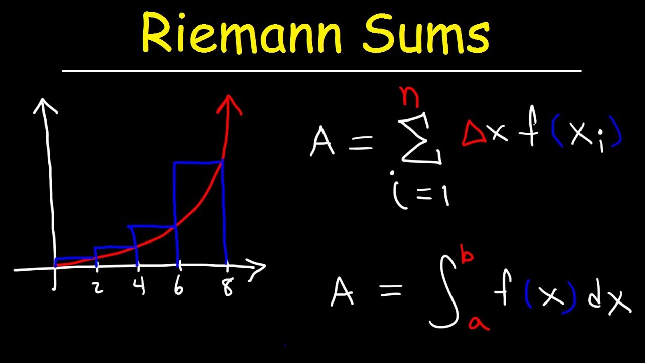
- 📏 Riemann sums involve creating rectangles under the curve with varying strategies for determining their heights, such as using left, right, or midpoint endpoints of intervals.
- 📉 The left Riemann sum uses the left endpoint of each interval to determine the height of the rectangle, which can lead to an overestimate or underestimate depending on the function's behavior.
- 📈 The right Riemann sum is similar but uses the right endpoint of the interval for the rectangle's height, which can also result in overestimation or underestimation.
- 🔄 The midpoint Riemann sum calculates the height of the rectangle at the midpoint of each interval, which can balance out the overestimations and underestimations to some extent.
- 🔽 The trapezoidal sum uses trapezoids instead of rectangles to approximate the area, taking the average of the left and right function values at the interval endpoints to determine the trapezoid's bases.
- ⏹ The concavity of the function affects the accuracy of the trapezoidal sum; concave down functions result in underestimates, while concave up functions lead to overestimates.
- 📉 The video demonstrates that as the width of the rectangles or trapezoids decreases (i.e., using more and smaller intervals), the approximation becomes more accurate, approaching the actual area under the curve.
- 📈 The script also covers how the sign of the function values (whether they are above or below the x-axis) affects the calculation, with areas below the x-axis contributing negatively to the total signed area.
- 🔢 The video provides examples using a given function and table values, illustrating the step-by-step process of applying Riemann and trapezoidal sums to approximate the area under the curve.
- 📝 The connection between the definite integral and the area under the curve is made, with the script showing how to approximate an integral using a midpoint sum with a given set of intervals.
Q & A
What is the main topic of the video?
-The main topic of the video is to demonstrate how to use Riemann and trapezoidal sums to approximate the area under a curve on a given interval.
What is the 'area under a curve' referring to in the context of the video?
-The 'area under a curve' refers to the area between the curve and the x-axis over a specified interval, which is the region the video aims to approximate using different summation techniques.
What are the different types of Riemann sums discussed in the video?
-The video discusses three types of Riemann sums: left Riemann sum, right Riemann sum, and midpoint Riemann sum.
How does the width of the rectangles used in Riemann sums affect the approximation?
-Reducing the width of the rectangles in Riemann sums results in a more accurate approximation of the area under the curve, as it minimizes the error between the rectangles and the actual curve.
What is the trapezoidal sum and how does it differ from Riemann sums?
-The trapezoidal sum is a method of approximating the area under a curve by using trapezoids instead of rectangles. Unlike Riemann sums, which use function values at specific points to determine the height of rectangles, trapezoidal sums calculate the area by averaging the function values at the endpoints of each sub-interval and multiplying by the width.
How does the concavity of a function affect the accuracy of the trapezoidal sum?
-If the function is concave down, the trapezoidal sum tends to underestimate the area, as each trapezoid captures less area than the actual curve. Conversely, if the function is concave up, the trapezoidal sum overestimates the area.
What is the purpose of using the left endpoint in a left Riemann sum?
-In a left Riemann sum, the left endpoint of each sub-interval is used to determine the height of the rectangle, which is then used to approximate the area under the curve on that sub-interval.
What is the effect of using a right Riemann sum on the approximation of the area under a curve?
-A right Riemann sum uses the right endpoint of each sub-interval to determine the height of the rectangle. This method tends to give an overestimate when the function is increasing and an underestimate when the function is decreasing.
How does the midpoint Riemann sum compare to the left and right Riemann sums in terms of accuracy?
-The midpoint Riemann sum often provides a more balanced approximation, as the rectangles' heights are determined by the midpoint values of the sub-intervals. This method tends to balance out the overestimations and underestimations that occur with left and right Riemann sums.
What is the connection between the area under the curve and the definite integral discussed in the video?
-The area under the curve, as approximated by methods like Riemann and trapezoidal sums, is directly related to the concept of the definite integral. The definite integral represents the exact area under the curve over a given interval, while the summation techniques provide numerical approximations of this area.
Outlines
📊 Introduction to Area Approximation Techniques
Michelle Kremmel introduces the concept of using Riemann and trapezoidal sums to approximate the area under a curve between the x-axis and the curve itself over a specified interval. She explains that instead of counting squares, rectangles of a systematic width are created and their areas are summed up to estimate the total area. The process involves ignoring parts of the graph outside the interval and focusing on the specific region between x=1 and x=7. The method begins with rectangles of width two, and the height of each rectangle is determined by the function value at the left edge of the rectangle where it intersects the curve. The areas of the rectangles are then computed and summed to give an approximation of the total area, which in this case is 42.667, representing a rough estimate rather than the exact area.
📐 Understanding Left Riemann Sums and Their Limitations
The script delves into the specifics of the left Riemann sum method, where the left endpoint of each subinterval is used to determine the height of the rectangles. It acknowledges the imperfect nature of this approximation, as some rectangles may extend outside the curve, leading to an overestimation in some areas and an underestimation in others. The process is repeated with narrower rectangles (width of one) to improve the approximation, resulting in an estimated area of 41.667. The script also discusses the impact of reducing the width of the rectangles, noting that it leads to a more accurate approximation. Additionally, it explains that a left Riemann sum tends to underestimate the area when the function is increasing and overestimate when the function is decreasing.
📉 Right Riemann Sums and Their Impact on Area Estimation
The video script shifts focus to the right Riemann sum, where the right endpoint of each subinterval is used to determine the height of the rectangles. This method results in a different approximation, with an initial estimate of 34.667, which is visually identified as an underestimate. The script explains that using narrower rectangles with a width of one leads to a more accurate approximation of 37.667. It also discusses the trade-off between the accuracy of the approximation and the complexity of the calculation, especially as the number of rectangles increases. The right Riemann sum is shown to underestimate when the function is decreasing and overestimate when the function is increasing, with the actual area lying between the estimates provided by the left and right Riemann sums.
🔍 Exploring Midpoint Riemann Sums for Balanced Approximations
The midpoint Riemann sum is introduced as a technique that uses the midpoint of each subinterval to determine the height of the rectangles. This method is shown to balance the surplus and deficit areas of the rectangles, providing a more accurate approximation of the area under the curve. The script illustrates this with rectangles of width two, resulting in an estimated area of 40.667. It emphasizes that making the width of the rectangles smaller improves the approximation, as demonstrated with widths of one and 0.5, yielding estimates of 40.167 and 40.042, respectively. The midpoint Riemann sum is noted for its balanced approach, although it's not as clear whether the approximation is an overestimate or an underestimate as it is with the left or right Riemann sums.
📈 Transitioning to Trapezoidal Sums for Area Approximation
The script introduces the trapezoidal sum as a new technique for approximating the area under a curve. Unlike the Riemann sums that use rectangles, the trapezoidal sum uses trapezoids formed by connecting the left and right endpoints of each subinterval to the curve. The area of each trapezoid is calculated as the average of the two bases (function values at the endpoints) times the height (width of the subinterval). The script demonstrates this method with subintervals of width two, resulting in an estimated area of 38.667. It notes that each trapezoid underestimates the actual area, regardless of whether the function is increasing or decreasing, and attributes this to the concavity of the function. The trapezoidal sum is shown to provide a better approximation when using narrower subintervals, with an estimate of 39.667 for width 0.5.
📚 Practical Application of Approximation Techniques
The video script provides practical examples of using the different approximation techniques with a given function, f(x), and its table values. It demonstrates how to apply the left Riemann sum, right Riemann sum, midpoint Riemann sum, and trapezoidal sum to approximate the area under the curve on the interval from 0 to 5. The script emphasizes the importance of understanding the function's behavior to determine whether the approximation is an overestimate or an underestimate. It also highlights the visual aspect of using a graph to verify the results and the algebraic process of calculating the areas of the rectangles or trapezoids for each method.
📉 Dealing with Functions that Cross the X-Axis
The script addresses the complexities that arise when approximating areas under a curve that crosses the x-axis, resulting in portions of the graph being above and below the x-axis. It explains that the height of the rectangles can be zero if the function value at an endpoint is at an x-intercept, leading to rectangles with no area. The script also discusses how to handle subintervals where the function is below the x-axis, using negative values for the heights of the rectangles and emphasizing the concept of signed area to account for regions below the x-axis.
🔗 Connecting Area Approximation to Definite Integrals
The final part of the script makes a connection between the area approximation techniques and definite integrals, which are a fundamental concept in calculus. Using a table of values, the script demonstrates how to approximate the integral of f(x) from 0 to 25 using a midpoint sum with three subintervals of varying widths. It shows the process of calculating the function values at the midpoints, determining the signed areas for each subinterval, and summing these to approximate the integral. The script concludes by emphasizing that the area calculated can be negative, which is represented as the signed area, and that this signed area corresponds to the definite integral.
👋 Closing Remarks and Future Lessons
In the closing paragraph, the presenter thanks the viewers for joining and expresses her anticipation for the next lesson. She hints at further exploration of the notation and concepts introduced in the video, indicating that more detailed explanations will be provided in the second part of the lesson. The presenter's sign-off is warm and inviting, setting the stage for continued learning and engagement in future sessions.
Mindmap
Keywords
💡Riemann Sum
💡Trapezoidal Sum
💡Area Under the Curve
💡Left Riemann Sum
💡Right Riemann Sum
💡Midpoint Riemann Sum
💡Concavity
💡Subinterval
💡Definite Integral
💡Signed Area
Highlights
Introduction to using Riemann and trapezoidal sums for approximating areas under a curve.
Explanation of the concept of 'area under a curve' as the region between the curve and the x-axis.
Demonstration of creating rectangles to systematically approximate the area under a curve.
Use of rectangles with a width of two to estimate the area between x=1 and x=7.
Description of the left Riemann sum technique using the left endpoint of subintervals to determine rectangle height.
Calculation of the area of rectangles to approximate the integral value, resulting in 42.667.
Switching to rectangles with a width of one for a more refined approximation.
Visual comparison of approximation accuracy with different rectangle widths.
Transition to using a right Riemann sum, utilizing the right endpoint of subintervals.
Observation that a right Riemann sum can lead to an underestimate or overestimate depending on the function's behavior.
Introduction of the midpoint Riemann sum, averaging the area captured by rectangles.
Comparison of midpoint Riemann sum results with varying rectangle widths.
Discussion on the difficulty of determining whether the midpoint Riemann sum results in an overestimate or underestimate.
Introduction of the trapezoidal sum method for area approximation.
Explanation of the trapezoidal sum's reliance on the concavity of the function to determine overestimation or underestimation.
Practice problems illustrating the application of different summation techniques with given function equations and table values.
Connection between the area under the curve and the definite integral, with an example of approximating an integral using a midpoint sum.
Final thoughts on the importance of understanding the behavior of functions and the impact on approximation techniques.
Transcripts
Browse More Related Video

Integration and Area under a Curve

AP Calculus AB - 6.2 Approximating Areas with Riemann Sums
Riemann Sums - Left Endpoints and Right Endpoints
Worked example: over- and under-estimation of Riemann sums | AP Calculus AB | Khan Academy
Calculus AB/BC – 6.2 Approximating Areas with Riemann Sums

Riemann and Trapezoidal Sums from Tables of Values
5.0 / 5 (0 votes)
Thanks for rating: