Calculus AB/BC – 6.2 Approximating Areas with Riemann Sums

The Algebros

7 Dec 202028:02

EducationalLearning

32 Likes 10 Comments

TLDRIn this informative lesson, Mr. Bean explores various methods for approximating the area under a curve, focusing on parabolas and intervals from 2 to 6 and 2 to 8. He introduces left and right Riemann sums, midpoint approximation, and trapezoidal sum, demonstrating how these techniques offer increasingly accurate estimates. The lesson also covers how to handle tables of values and the impact of a function's concavity on the accuracy of the approximations. Understanding whether the function is increasing or decreasing is crucial for determining if the approximation is an overestimate or underestimate.

Takeaways

📚 The concept of approximating the area under a curve using various methods is introduced, specifically when dealing with shapes that do not have simple geometric forms.
📈 The lesson focuses on parabolas and the interval from 2 to 6 as an example for approximation.
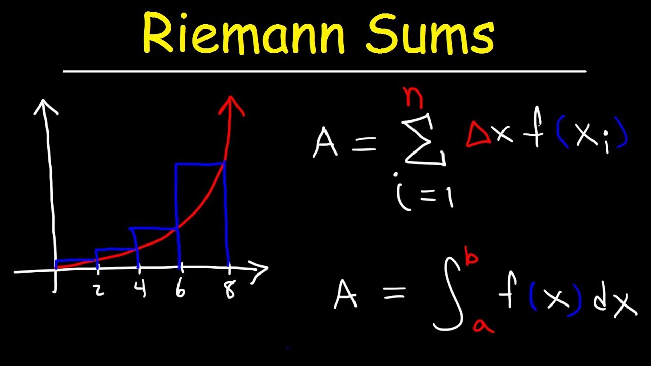
📊 Left, right, and midpoint Riemann sums are explained as methods to approximate the area under a curve by breaking it into rectangles or strips.
🔢 The width of each rectangle in the Riemann sums is determined by the interval and the number of sub-intervals chosen.
🖼️ Riemann sums involve creating rectangles that touch the curve at specific points (left, right, or midpoint) to calculate the area.
📐 The trapezoidal rule is introduced as a more accurate method for approximation, which involves creating trapezoids by connecting the points at the intervals.
📈 The accuracy of the approximation increases with the number of sub-intervals used in the Riemann sums.
🔄 The process of estimating the area under a curve can be visualized by sketching the rectangles or trapezoids on the graph.
📝 Tables of values are used to simplify the process of approximation when only specific data points are given, rather than the full function.
📊 The script provides examples of how to calculate the area using left, right, midpoint, and trapezoidal approximations with a given set of values.
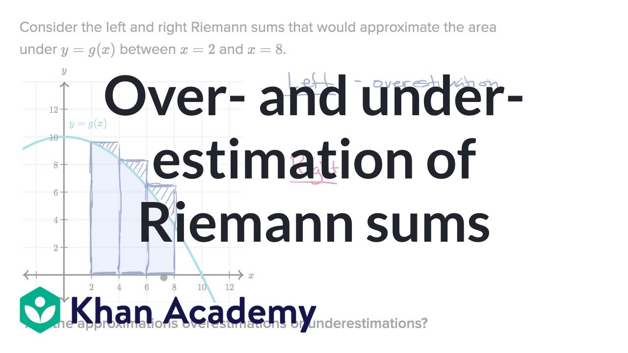
🔍 The script also discusses how to determine whether the approximation is an overestimate or underestimate based on the function's concavity and the type of Riemann sum used.

Q & A

What is the main topic of the lesson?
-The main topic of the lesson is approximating the area under a curve, specifically using Riemann sums and various approximation methods for different types of functions.
How does Mr. Bean introduce the concept of approximating areas under curves?
-Mr. Bean introduces the concept by discussing the difficulty of finding the area under a curve that does not have a simple geometric shape, such as a parabola, and then explains that approximation methods can be used to estimate these areas.
What is the first approximation method discussed in the lesson?
-The first approximation method discussed is the left rectangle approximation, where rectangles are created on the interval with the left side touching the curve, providing an approximation of the area under the curve.
How does the number of sub-intervals (n) affect the approximation?
-The number of sub-intervals (n) determines the width of each rectangle used in the approximation. As n increases, the width of each rectangle decreases, leading to a more accurate approximation of the area under the curve.
What is a Riemann sum and how is it related to approximating areas under curves?
-A Riemann sum is the result of adding up the areas of rectangles (or other shapes) created on sub-intervals of the curve. It is used as an approximation for the exact area under the curve, with the accuracy improving as more sub-intervals are used.
What are the three types of Riemann sums discussed in the lesson?
-The three types of Riemann sums discussed are the left Riemann sum, the right Riemann sum, and the midpoint Riemann sum. Each involves calculating the area of rectangles in a different way to approximate the area under the curve.
How does the shape of the function (increasing or decreasing) and the type of Riemann sum (left, right, or midpoint) affect the accuracy of the approximation?
-The accuracy of the approximation depends on whether the function is increasing or decreasing and which type of Riemann sum is used. For example, a left Riemann sum on an increasing function will underestimate the area, while a right Riemann sum will overestimate it. The midpoint Riemann sum provides a more balanced approximation.
What is the trapezoidal rule mentioned in the lesson?
-The trapezoidal rule is a method for approximating the area under a curve by breaking it into trapezoids. It is considered more accurate than the Riemann sum methods because it accounts for the change in slope within each sub-interval, leading to a better fit of the geometric shapes to the curve.
How does the lesson use a table of values to calculate Riemann sums?
-The lesson demonstrates how to use a table of values to determine the height (y-value) of rectangles or trapezoids at specific x-values within each sub-interval. This allows for the calculation of the area of each shape and the summation of these areas to approximate the total area under the curve.
What is the significance of the concavity of a function in relation to the trapezoidal rule?
-The concavity of a function affects whether the trapezoidal rule will overestimate or underestimate the area under the curve. If the function is concave up, the trapezoidal rule will overestimate the area, and if it is concave down, the rule will underestimate the area.
How does the lesson conclude regarding the accuracy of the approximation methods?
-The lesson concludes that while all the methods discussed are approximations, the accuracy can be improved by increasing the number of sub-intervals used. It also emphasizes the importance of understanding the function's behavior (increasing/decreasing, concavity) to determine whether an approximation is likely to be an overestimate or an underestimate.

Outlines

00:00

📚 Introduction to Approximating Under Curve Area

The paragraph introduces the concept of approximating the area under a curve, specifically focusing on non-geometric shapes like a parabola. Mr. Bean explains the process of using approximation methods to find the area under a curve from 2 to 6, highlighting the transition from simple geometric shapes to more complex functions. The explanation includes the initial steps of breaking down the process into sub-intervals and the introduction of the left rectangle approximation method.

05:01

📈 Left Riemann Sum and Sub-Intervals

This section delves into the specifics of performing a left Riemann sum, including the calculation of sub-intervals and the width of rectangles used for approximation. The process is demonstrated with a function from 2 to 8, and the calculation is shown for three sub-intervals. The concept of increasing or decreasing functions and their impact on overestimation or underestimation is also briefly touched upon, setting the stage for further exploration in subsequent paragraphs.

10:03

📊 Midpoint and Trapezoidal Approximations

The paragraph discusses the midpoint and trapezoidal approximations for finding the area under a curve. It explains how to calculate the height of the rectangles at the midpoint and how to create trapezoids by connecting the points on the curve. The paragraph emphasizes the accuracy of trapezoidal approximations over simpler methods and provides a step-by-step guide on how to perform these calculations.

15:04

🔢 Riemann Sums with Tables of Values

This section introduces the application of Riemann sums using a table of values, which simplifies the process by providing specific data points. The example given involves calculating the rate of change over a 12-minute interval, using both left and right Riemann sums to estimate the amount of gallons pumped into a tank. The paragraph also discusses the implications of the function's increasing or decreasing nature on the accuracy of the estimates.

20:05

📋 Estimating with Midpoints and Trapezoids from a Table

The final paragraph focuses on applying midpoint and trapezoidal approximations using values from a table. It explains how to calculate the area using the midpoint method by taking the average of the y-values within each sub-interval. The trapezoidal method is also covered, detailing how to find the average height of two points and multiply it by the width of the interval. The paragraph concludes with a comparison of the estimates from different methods, providing insights into their relative accuracy.

Mindmap

Keywords

💡Riemann Sum

A Riemann Sum is a method used to approximate the area under a curve when the shape is not a simple geometric figure. It involves breaking the area into smaller, more manageable parts, typically rectangles or trapezoids, and calculating the area of each part to estimate the total area. In the video, Mr. Bean uses Riemann Sums to approximate the area under a parabola, demonstrating left, right, and midpoint approximations as well as trapezoidal sums.

💡Left Riemann Sum

A Left Riemann Sum is a technique where rectangles are constructed to approximate the area under a curve by using the leftmost point of each subinterval to determine the height of the rectangles. This method tends to underestimate the actual area, especially for increasing functions, because it does not account for the entire area under the curve.

💡Right Riemann Sum

A Right Riemann Sum is a method where rectangles are created using the rightmost point of each subinterval to determine the height of the rectangles. This approach can overestimate the actual area, particularly for increasing functions, because it includes extra space beyond the curve.

💡Midpoint Riemann Sum

A Midpoint Riemann Sum is an approximation technique where the midpoint of each subinterval is used to determine the height of the rectangles. This method provides a balance between underestimation and overestimation, offering a more accurate approximation of the area under the curve compared to left or right Riemann sums.

💡Trapezoidal Sum

A Trapezoidal Sum is an advanced Riemann Sum technique that involves breaking the area under the curve into trapezoids and calculating their areas. This method is more accurate than simple Riemann sums because it accounts for the curvature of the function within each subinterval, providing a closer approximation to the true area.

💡Approximation

In mathematics, approximation refers to the process of estimating a value or quantity that is not exactly known or cannot be precisely calculated. In the context of the video, approximation is used to estimate the area under a curve when it cannot be easily determined using basic geometric formulas.

💡Parabolas

A parabola is a U-shaped curve that is symmetrical about its axis and has a single maximum or minimum point. In the video, Mr. Bean uses a parabola as an example to demonstrate how to approximate the area under a curve that does not have a simple geometric shape.

💡Subintervals

Subintervals are smaller segments of a larger interval on the number line. In the context of approximating areas under curves, subintervals are used to divide the area into smaller, more manageable parts that can be approximated using rectangles or trapezoids.

💡Area

In mathematics, the term 'area' refers to the amount of space enclosed within a two-dimensional shape. The video focuses on approximating the area under a curve, which is a more complex shape than traditional geometric figures.

💡Width and Height

In the context of the video, 'width' and 'height' are used to describe the dimensions of the rectangles or trapezoids used in the approximation methods. The width corresponds to the length of the subinterval on the x-axis, while the height is determined by the function's value at specific points on the y-axis.

💡Table of Values

A table of values is a list of numerical data points that show the relationship between the input (independent variable) and the output (dependent variable) for a given function. In the video, a table of values is used to provide specific points on the curve to assist in approximating the area under it.

Highlights

Introduction to approximating the area under a curve using methods other than simple geometric shapes.

Explanation of breaking down a parabolic curve into subintervals for approximation.

Description of left rectangle approximation and its process.

Demonstration of how increasing the number of subintervals improves the approximation.

Introduction to Riemann sums and their use in approximating areas under curves.

Detailed walk-through of calculating a left Riemann sum with a given function.

Explanation of right Riemann sums and how they differ from left Riemann sums.

Step-by-step calculation of a midpoint Riemann sum and its simplification.

Discussion on the accuracy of different Riemann sum methods and how they compare.

Introduction to trapezoidal sums as a more accurate approximation method.

Illustration of how to calculate trapezoidal sums using given data points.

Explanation of how the concavity of a function affects the accuracy of trapezoidal sums.

Application of Riemann sums to a real-world problem involving rate of change and accumulation of change.

Demonstration of using a table of values to simplify Riemann sum calculations.

Comparison of different Riemann sum methods using a table of values to find an approximate answer.

Conclusion on the effectiveness of Riemann sums in approximating areas under curves and their practical applications.

Transcripts

Browse More Related Video

AP Calculus AB - 6.2 Approximating Areas with Riemann Sums

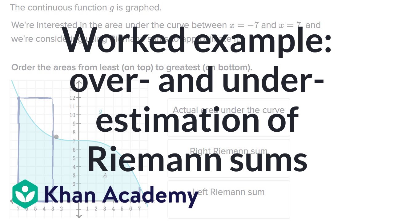
Worked example: over- and under-estimation of Riemann sums | AP Calculus AB | Khan Academy

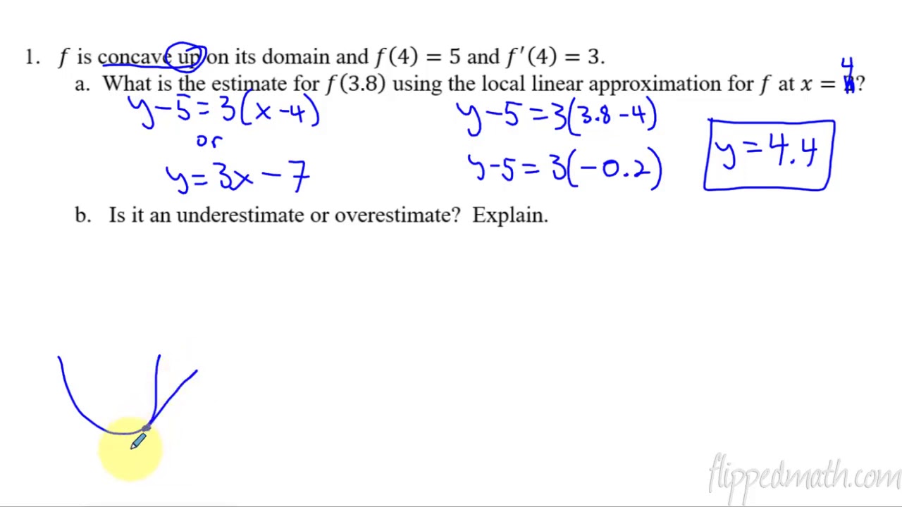
Calculus AB/BC – 4.6 Approximating Values of a Function Using Local Linearity and Linearization

AP Calculus AB: Lesson 6.2 Riemann and Trapezoidal Sums

Riemann Sums - Left Endpoints and Right Endpoints

Over- and under-estimation of Riemann sums | AP Calculus AB | Khan Academy

Related Tags

Mathematics Calculus Riemann Sums Area Approximation Parabolic Curves Mr. Bean Educational Content Tutorial Geometry Numerical Analysis