Worked example: over- and under-estimation of Riemann sums | AP Calculus AB | Khan Academy
TLDRThe video script discusses the use of Riemann sums to approximate the area under a continuous function's curve between specific x-values. It explains the concept of left and right Riemann sums, using examples and illustrations to show how they can overestimate or underestimate the actual area. The video encourages viewers to visualize and understand the process of approximating areas using these methods, highlighting the importance of accurate subdivision selection for better approximation.
Takeaways
- 📈 The script discusses using Riemann sums to approximate the area under a continuous function's curve.
- 🔢 It highlights the process of calculating the area between x = -7 and x = 7 using Riemann sums.
- 🖌️ The video includes a visual representation from a Khan Academy exercise for better understanding.
- 🔄 The concept of ordering areas from least to greatest is introduced, with 1 being the least and 3 the greatest.
- 📏 The script explains the concept of left Riemann sums and how they are calculated using the left endpoint of each subdivision.
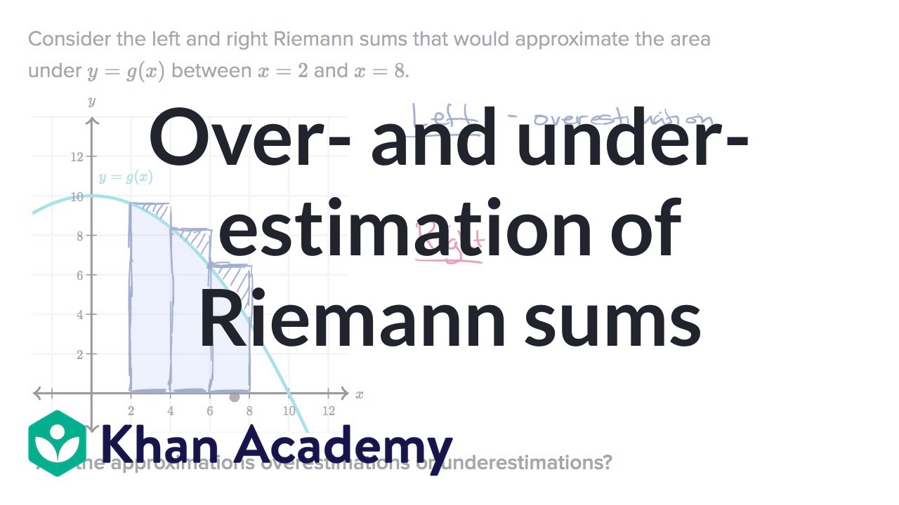
- 📈 The left Riemann sum is noted to be an overestimate of the actual area under the curve due to the function's nature of not increasing.
- 📏 The concept of right Riemann sums is also discussed, with the height of rectangles determined by the right endpoint's function value.
- 🔄 The right Riemann sum is shown to be an underestimate of the actual area, as the function is either decreasing or flat.
- 🏆 The actual area of the curve is considered the most accurate and is placed in the middle when ranking the estimates.
- 🔢 A comparison between the left Riemann sum (overestimate), the actual area, and the right Riemann sum (underestimate) is provided.
- 📊 The script encourages doing fewer subdivisions for a general sense of the approximation and acknowledges that subdivisions don't have to be equal.
Q & A
What is the main topic discussed in the video?
-The main topic discussed in the video is the use of Riemann sums to approximate the area under a continuous function's curve between two given points.
What is the area of interest in the video?
-The area of interest in the video is the area under the curve of a continuous function, specifically between x equals negative seven and x equals seven.
What is the purpose of using Riemann sums in this context?
-The purpose of using Riemann sums in this context is to estimate the area under the curve of a continuous function between two points, which can be challenging to calculate directly.
How does the video demonstrate the use of Riemann sums?
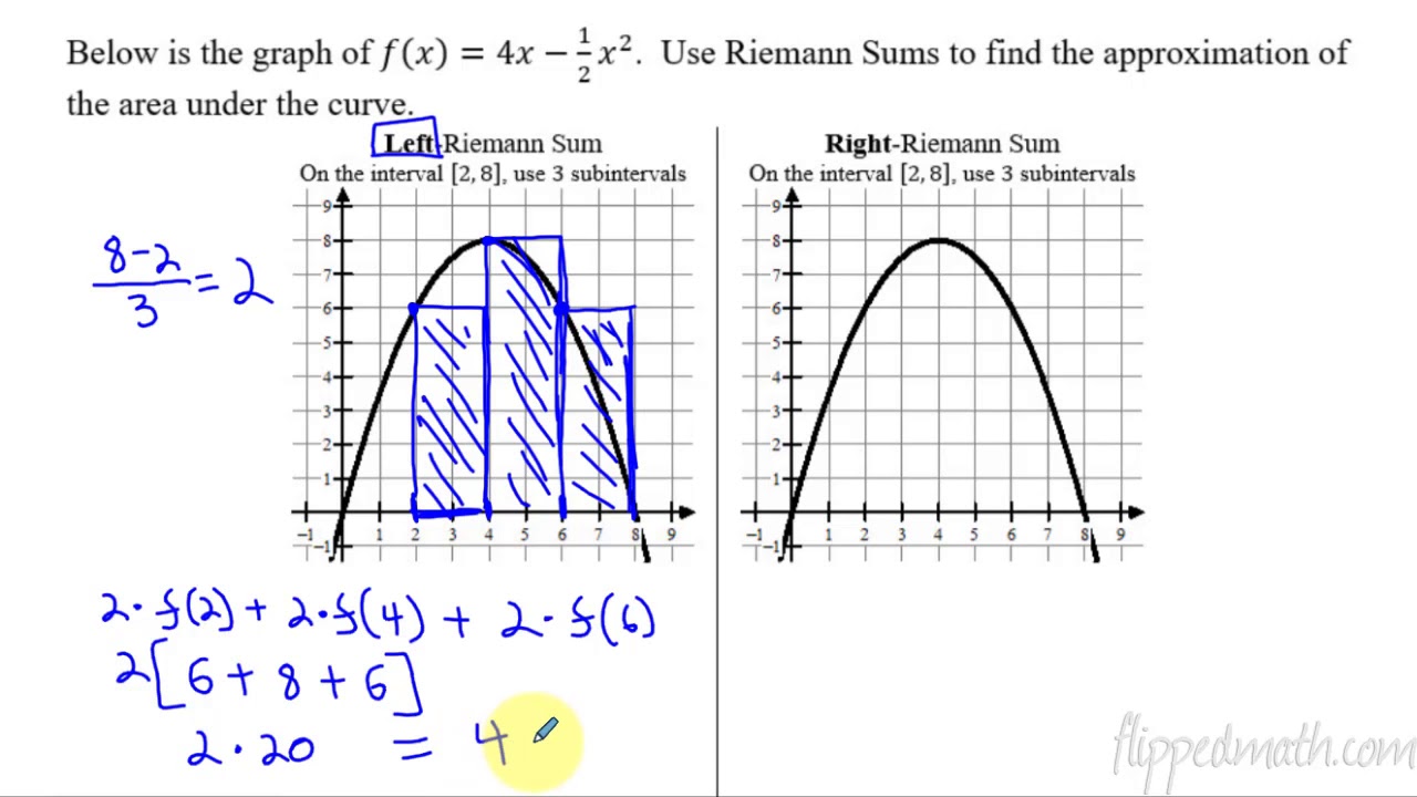
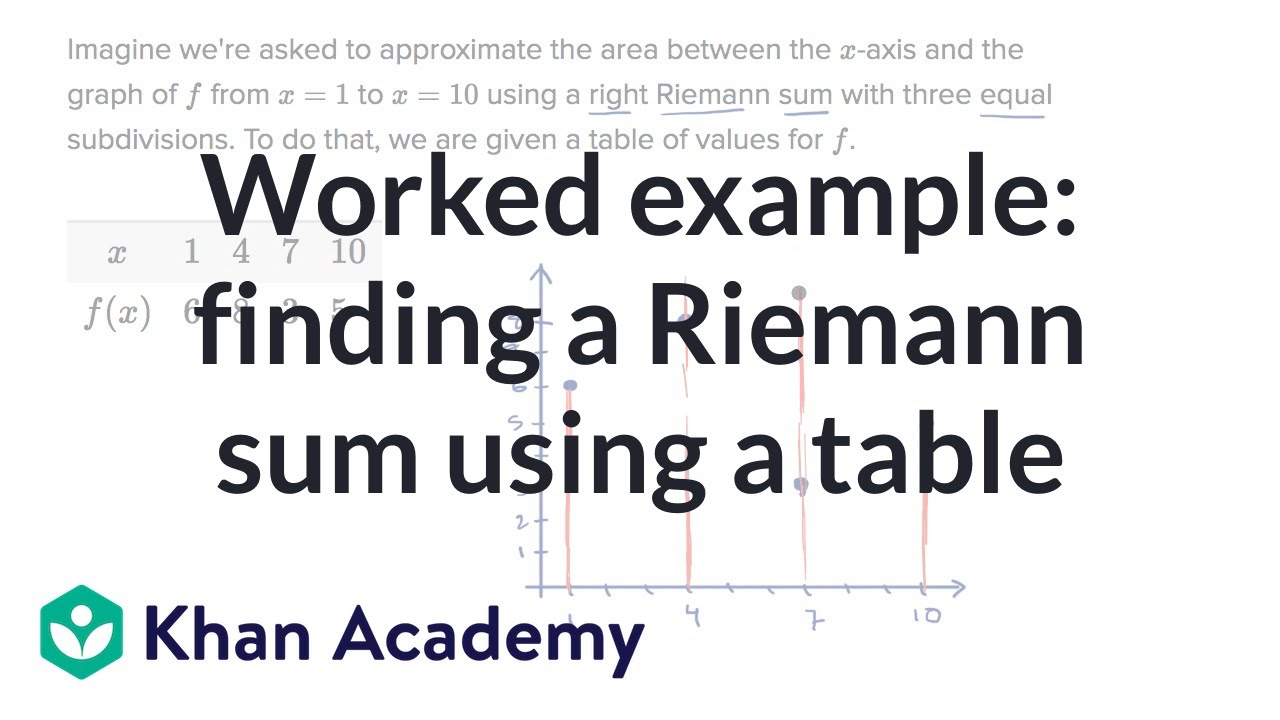
-The video demonstrates the use of Riemann sums by showing how to divide the area of interest into smaller rectangles, using either the left or right endpoint of each subdivision to estimate the area under the curve.
What is the difference between a left Riemann sum and a right Riemann sum?
-A left Riemann sum uses the value of the function at the left endpoint of each subdivision to estimate the area, while a right Riemann sum uses the value of the function at the right endpoint of each subdivision.
Why does the left Riemann sum overestimate the actual area under the curve?
-The left Riemann sum overestimates the actual area because the function is either decreasing or flat, so the value at the left endpoint is as high or higher than any other value within that interval, leading to extra area being included in the estimation.
Why does the right Riemann sum underestimate the actual area under the curve?
-The right Riemann sum underestimates the actual area because the function is either decreasing or flat, so the value at the right endpoint is smaller and thus continuously misses out on including some area under the curve.
How can the accuracy of Riemann sums be improved?
-The accuracy of Riemann sums can be improved by increasing the number of subdivisions, which allows for a more precise approximation of the area under the curve.
What is the relationship between the Riemann sums, the actual area, and the ranking from least to greatest?
-The right Riemann sum is the least as it underestimates the area, followed by the actual area of the curve, and then the left Riemann sum which is the greatest as it overestimates the area.
How does the video encourage the viewer to engage with the material?
-The video encourages the viewer to engage with the material by pausing at key points to allow the viewer to think about and rank the different estimations of the area under the curve.
What is the significance of the function's behavior in determining whether Riemann sums will overestimate or underestimate the area?
-The function's behavior, specifically whether it is increasing, decreasing, or constant, significantly impacts whether Riemann sums will overestimate or underestimate the area. For a decreasing or constant function, left Riemann sums will overestimate and right Riemann sums will underestimate the area.
Outlines
📊 Understanding Riemann Sums and Area Estimations
The paragraph discusses the concept of using Riemann sums to approximate the area under a continuous function's curve. The focus is on the function g, and the area of interest is between x = -7 and x = 7. The instructor explains the process of ordering the areas from least to greatest and introduces a visual representation from a Khan Academy exercise. The concept of left and right Riemann sums is introduced, with examples provided for both. The left Riemann sum is noted to overestimate the area, as it uses the function value at the left end of each subdivision, which is higher or equal to other values in that interval. Conversely, the right Riemann sum is shown to underestimate the area, as it uses the function value at the right end of each subdivision, which is smaller or equal to other values in that interval. The paragraph concludes with a ranking of the approximations from least (right Riemann sum) to greatest (left Riemann sum), in comparison to the actual area under the curve.
Mindmap
Keywords
💡Continuous Function
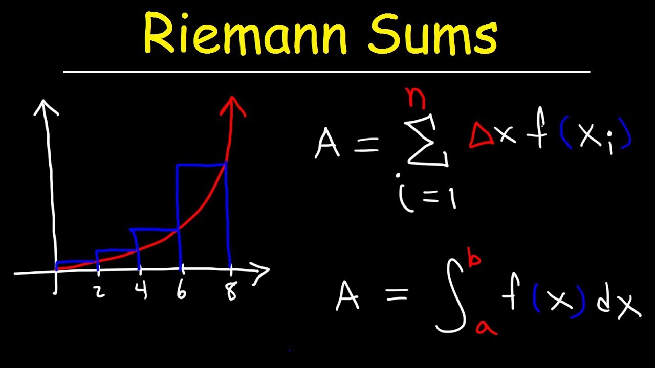
💡Riemann Sums
💡Area Under the Curve
💡Subdivisions
💡Left Riemann Sum
💡Right Riemann Sum
💡Overestimate and Underestimate
💡Khan Academy Exercise
💡Unequal Subdivisions
💡Function Value
💡Graph
Highlights
The continuous function g is graphed and the area under the curve between x equals negative seven and x equals seven is of interest.
Riemann sums are suggested as a method to approximate the area under the curve.
The concept of ordering areas from least to greatest is introduced, with a visual representation in different colors.
A screenshot from a Khan Academy exercise is mentioned, where users would interact with a graphical representation.
The process of ordering the areas from least to greatest is demonstrated by writing numbers and considering their positions.
A left Riemann sum is explained, starting at x equals negative seven and going to x equals seven.
The first rectangle of the left Riemann sum is defined by the value of the function at x equals negative seven, which is 12.
It is noted that the left Riemann sum is an overestimate relative to the actual area.
The concept of subdivisions in Riemann sums is discussed, with an emphasis on not needing equal subdivisions.
The second and third subdivisions of the left Riemann sum are described, with the height of rectangles determined by the function's value at the left end.
The reason why the left Riemann sum is an overestimate is explained, relating to the function's behavior of not increasing.
A right Riemann sum is introduced, with different subdivisions and the use of the right edge to define the height.
The first rectangle of the right Riemann sum is defined using the value of the function at the right edge, x equals negative five.
The right Riemann sum is described as an underestimate of the area under the curve.
The rectangles in the right Riemann sum are continuously underestimating the area, as the function's value at the right edge is smaller.
The ranking of the areas from least to greatest is provided, with the right Riemann sum as the least, the actual area of the curve in the middle, and the left Riemann sum as the greatest.
Transcripts
Browse More Related Video
Over- and under-estimation of Riemann sums | AP Calculus AB | Khan Academy
Calculus AB/BC – 6.2 Approximating Areas with Riemann Sums

AP Calculus AB: Lesson 6.2 Riemann and Trapezoidal Sums

AP Calculus AB - 6.2 Approximating Areas with Riemann Sums
Worked example: finding a Riemann sum using a table | AP Calculus AB | Khan Academy
Riemann Sums - Left Endpoints and Right Endpoints
5.0 / 5 (0 votes)
Thanks for rating: