Statistics Lecture 3.2: Finding the Center of a Data Set. Mean, Median, Mode

Professor Leonard

8 Dec 201171:27

EducationalLearning

32 Likes 10 Comments

TLDRThis educational video script delves into the concepts of data description, focusing on the center and variation of datasets. It introduces the mean, median, and mode as measures of central tendency, explaining their calculation and application. The script also addresses the impact of outliers and the importance of data distribution, including normal and skewed distributions. It further explains how to calculate the mean of a frequency distribution and a weighted distribution, providing formulas and examples. The presenter uses a step-by-step approach to guide learners through the process, ensuring a comprehensive understanding of these fundamental statistical concepts.

Takeaways

📊 The script discusses five key characteristics for describing data, focusing initially on the center and variation of data sets.
🔢 The center of data is described using three common measures: mean (average), median (middle value), and mode (most frequently occurring value).
🧩 The mean is calculated by adding all data values together and dividing by the number of values, symbolized as \( \bar{X} \) for sample mean and \( \mu \) for population mean.
📈 The median is the middle value of a data set when ordered from smallest to largest and is less affected by outliers compared to the mean.
📚 The mode is the most frequently occurring value in a data set and can be unimodal (one mode), bimodal (two modes), multimodal (more than two modes), or no mode at all.
🚫 Outliers are data points that are significantly different from other observations and can skew the mean, but do not affect the median as much.
📉 Skewness refers to the asymmetry of the data distribution, which can be skewed to the right (larger outliers) or skewed to the left (smaller outliers).
📚 The script also covers calculating the mean of a frequency distribution, which involves multiplying the midpoint of each class by its frequency and then summing these products.
🔄 The process of calculating a weighted mean is explained, which involves multiplying each score by its respective weight and then summing these products to find the overall mean.
🔢 The rounding rule in statistics is highlighted, emphasizing that numbers should be rounded to one more decimal place than the original data and not rounded until the final step of a calculation.
📱 The use of a calculator to find mean, median, mode, and other statistics is demonstrated, showcasing the ease and efficiency of using technology for statistical calculations.

Q & A

What are the five characteristics of describing data discussed in the script?
-The five characteristics of describing data discussed in the script are the center of the data, variation, distribution, outliers, and changes over time.
What is the center of the data in the context of the script?
-The center of the data refers to the middle or the most frequent value of the dataset, which is often represented by measures such as the mean, median, and mode.
What does the script mean by 'variation' when describing data?
-Variation refers to how the data changes, including the distribution of the data and the presence of outliers, which are data points that are significantly different from the rest of the data set.
What is the mean and how is it calculated according to the script?
-The mean is the arithmetic average, calculated by adding up all the values in the dataset and dividing by the number of values. It is represented by the symbol μ for a population mean and x̄ for a sample mean.
What is the difference between a population mean (μ) and a sample mean (x̄) as described in the script?
-The population mean (μ) represents the mean of an entire population, while the sample mean (x̄) represents the mean of a subset of that population. They are calculated in the same way, but different symbols are used to distinguish between them.
How does the script explain the concept of the median?
-The median is explained as the middle value of a dataset. If the dataset has an odd number of values, the median is the middle number. If it has an even number of values, the median is the average of the two middle numbers.
What is the mode in statistics and how is it different from the mean and median?
-The mode is the most frequently occurring value in a dataset. It differs from the mean and median in that it focuses on the most common value, rather than the central tendency or the middle value of the dataset.
Why might median be used instead of mean, as hinted in the script?
-Median might be used instead of mean to avoid being affected by outliers or extreme values. Because median is the middle value in an ordered dataset, it is less sensitive to outliers, making it a more representative measure of central tendency in certain situations.
What is the concept of 'outliers' as discussed in the script?
-Outliers are data points that are significantly different or distant from other values in the dataset. They can skew the results of calculations like the mean, making it less representative of the majority of the data.
Can you provide an example of calculating the mean from the script?
-An example provided in the script for calculating the mean is adding up the ages of individuals in a classroom and then dividing by the total number of people to find the average age.
What is the rounding rule mentioned in the script and how should it be applied?
-The rounding rule mentioned in the script states that numbers should be rounded to one more decimal place than what is given. Additionally, rounding should not be done until the very last step of a calculation to avoid compounding errors.

Outlines

00:00

📊 Describing Data Characteristics

The video begins by introducing Chapter 3, which focuses on describing data through five key characteristics. The instructor emphasizes the importance of understanding the center of the data, which is the middle or most frequent value, and mentions the three common measures of central tendency: mean, median, and mode. The mean is defined as the arithmetic average, calculated by summing all values and dividing by the number of values. The video promises to cover variation, distribution, outliers, and changes over time in the subsequent parts.

05:11

🔢 Understanding the Mean

The instructor delves deeper into the concept of the mean, explaining it as the first measure of central tendency. Symbols and mathematical notation are introduced to represent the mean, with the lowercase 'n' for the number of values in a sample and the uppercase 'N' for a population. The mean is calculated by summing all values (denoted by the Greek letter Sigma) and dividing by the number of values. The notation for the sample mean is represented by 'X̄', and for the population mean by the Greek letter 'μ' (mu). The video illustrates the formula for calculating the mean and emphasizes its importance in understanding the center of a data set.

10:12

📈 Calculating and Interpreting the Mean

The video provides a practical example of calculating the mean using a sample data set. The data represents the amount of change in a car over several months, including an outlier of a large amount. The instructor guides the viewers through the process of summing the values and dividing by the number of data points to find the sample mean. The result is an expected value that most data points are close to, illustrating how the mean can be used to understand the central tendency of a data set.

15:13

🏠 Median as a Measure of Central Tendency

The video introduces the median as another measure of central tendency, which is the middle value of an ordered data set. The instructor explains that the median is less affected by outliers compared to the mean, making it a useful measure when data is skewed. The process of finding the median involves ordering the data from smallest to largest and identifying the middle value. If the data set has an even number of values, the median is calculated as the average of the two middle numbers.

20:14

📈 Impact of Outliers on Mean and Median

The instructor discusses the impact of outliers on the mean and median. An outlier is a data point that is significantly different from the rest of the data. While the mean can be greatly affected by outliers, the median remains relatively stable because it is based on the middle value of the ordered data. The video uses an example of a large outlier in a data set to demonstrate how it can significantly increase the mean but not affect the median, highlighting the robustness of the median in the presence of extreme values.

25:35

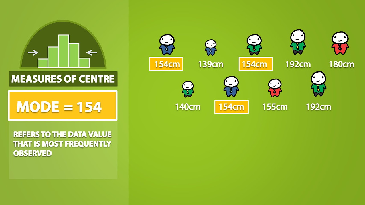
📊 Exploring the Mode and Rounding Rules

The video continues by explaining the mode, which is the most frequently occurring value in a data set. It can be unimodal (one mode), bimodal (two modes), multimodal (more than two modes), or have no mode at all. The instructor also introduces the concept of rounding rules in statistics, emphasizing the importance of not rounding until the very last step of a calculation to avoid magnifying errors.

30:36

📉 Calculating the Mean of a Frequency Distribution

The instructor demonstrates how to calculate the mean of a frequency distribution, which involves using midpoints of classes and multiplying them by their respective frequencies. This process yields an approximation of the mean because it assumes that all values within a class are represented by the class midpoint. The video provides a step-by-step guide on performing this calculation.

36:00

🎓 Weighted Mean and Understanding Skewness

The video concludes with an introduction to the weighted mean, which is used when different components of a data set have different levels of importance or 'weights'. The instructor explains how to calculate the weighted mean by multiplying each value by its corresponding weight and then summing these products. The mean is then found by dividing this sum by the total weight. Additionally, the concept of skewness is introduced, explaining how data can be skewed to the left or right due to the presence of outliers.

41:23

📚 Using a Calculator for Statistical Calculations

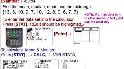
The final part of the video provides a tutorial on using a calculator to find mean, median, mode, and other statistical measures. The instructor guides viewers through entering data into the calculator's memory, accessing the statistical functions, and retrieving the calculated values. This segment aims to make the process of statistical analysis more efficient and accessible.

Mindmap

Keywords

💡Describing Data

Describing data refers to the process of summarizing and explaining the characteristics of a data set. In the video, this concept is central as it discusses various methods to quantify and understand data, such as finding the center, variation, distribution, and outliers. The script mentions five key things to consider when describing data, emphasizing the importance of these methods in understanding data behavior.

💡Center

The 'center' in the context of data refers to the middle or average value of a data set, which is a measure of central tendency. The script explains three common ways to describe the center: mean, median, and mode. The mean is the arithmetic average, the median is the middle value when data is ordered, and the mode is the most frequently occurring value. These measures are crucial for understanding where the bulk of the data lies.

💡Mean

The 'mean' is the arithmetic average of a data set, calculated by adding up all the values and dividing by the number of values. The script uses the mean to illustrate the concept of the center of data, explaining that it can be affected by outliers and is used to find the expected value in a data set. The mean is distinguished between a sample mean (denoted by X̄) and a population mean (denoted by μ).

💡Median

The 'median' is the value that separates a data set into two equal halves. If the number of data points is odd, the median is the middle number; if even, it is the average of the two middle numbers. The script points out that the median is less affected by outliers compared to the mean, making it a robust measure of central tendency.

💡Mode

The 'mode' is the value that occurs most frequently in a data set. A data set can have no mode, one mode (unimodal), two modes (bimodal), or more than two modes (multimodal). The script briefly touches on the mode as another way to describe the center of data, though it is less commonly used in the class's context.

💡Outliers

Outliers are data points that are significantly different from other observations, lying outside the normal range of a data set. The script discusses how outliers can skew the mean and affect the representation of data, which is why the median is often preferred in cases with significant outliers, such as in median household income or home values.

💡Variation

Variation refers to the differences or fluctuations in data points. The script mentions variation as one of the five things to consider when describing data. It is an important aspect because it gives insight into the spread or dispersion of the data around the center.

💡Distribution

The term 'distribution' in statistics refers to the way data points are spread out. The script discusses normal distribution, which is a symmetrical distribution often represented by a bell curve. It also mentions skewed distributions, where the data points are not symmetrically distributed, having more values on one side than the other.

💡Skewness

Skewness is a measure of the asymmetry of the probability distribution of a real-valued random variable. The script explains that if a distribution is skewed to the right, it has a tail that extends to the right, indicating larger outliers, while a skew to the left indicates smaller outliers. Understanding skewness is important for interpreting data correctly.

💡Weighted Mean

A 'weighted mean' is an average that takes into account the relative importance or 'weight' of each data point. In the script, the concept is used in the context of calculating grades in a class, where different components like homework, tests, and the final exam have different weights. The weighted mean is calculated by multiplying each value by its weight and then dividing by the sum of the weights.

💡Frequency Distribution

A 'frequency distribution' is a table or graph that displays the frequency or number of data points within different intervals or groups in a data set. The script explains how to calculate the mean of a frequency distribution, which involves using midpoints of the intervals and their corresponding frequencies to find an average that represents the entire data set.

Highlights

Introduction to Chapter 3 focusing on describing data through five key characteristics.

Explanation of the first characteristic, Center, as the middle or most frequent value in a data set.

Introduction of three common measures of central tendency: mean, median, and mode.

Detailed description of calculating the mean (average) as the arithmetic average of a data set.

Use of symbols and notation to represent the mean, including Σ (sum) and X̄ (sample mean).

Differentiation between sample mean (X̄) and population mean (μ), and their respective notations.

Procedure for calculating the median as the middle value of an ordered data set.

Explanation of how the median is affected by even and odd numbers of data points.

Illustration of the mean's sensitivity to outliers compared to the median's robustness.

Introduction and explanation of the mode as the most frequently occurring value in a data set.

Discussion on the concept of skewness and its impact on the distribution of data.

Demonstration of how to calculate mean, median, and mode using a graphing calculator.

Overview of creating and interpreting frequency distributions and their mean.

Calculation of weighted mean and its application in grading systems.

Explanation of how to convert different point scales into a percentage scale for calculating weighted mean.

Introduction to the concept of variation as the second characteristic of data.

Transcripts

Browse More Related Video

Mode, Median, Mean, Range, and Standard Deviation (1.3)

Elementary Statistics - Chapter 3 Describing Exploring Comparing Data Measure of Central Tendency

AP Psychology Statistics Simplified: Normal Distribution, Standard Deviation, Percentiles, Z-Scores

Math 119 Chapter 3 part 2

Elementary Stats Lesson #3 A

Statistics: Standard deviation | Descriptive statistics | Probability and Statistics | Khan Academy

Related Tags

Data Analysis Statistics Education Mean Calculation Median Mode Data Distribution Outliers Impact Weighted Mean Skewness Detection Frequency Distribution Educational Content