Elementary Stats Lesson #3 A
TLDRThis lesson covers descriptive statistics, focusing on measures of central tendency and spread in data sets. It explains how to calculate the mean, median, and mode, and introduces concepts like frequency tables, relative and cumulative frequencies. The lesson also highlights the importance of understanding outliers and skewness, and their impact on data summaries. Additionally, it demonstrates how to use a calculator for statistical analysis, including storing data, creating histograms, and calculating one-variable statistics. The concept of resistance in statistical measures and the introduction of standard deviation as a measure of spread are also discussed.
Takeaways
- 📚 The lesson introduces descriptive statistics as a way to analyze data sets with meaningful values, starting with frequency tables and histograms.
- 📈 The script discusses the importance of cumulative frequencies and relative frequencies for understanding the distribution of data points in a quiz score example.
- 🔢 The arithmetic mean, or simply the mean, is introduced as a measure of central tendency, calculated by summing all values and dividing by the number of observations.
- 💬 The notation for population mean is represented by the Greek letter mu (μ), while sample mean is denoted by x-bar (x̄), highlighting the difference between parameters and statistics.
- 🚫 The mean is noted to be not resistant to outliers and skewness, which can significantly impact its value, especially in small data sets.
- 🔄 The median is introduced as a resistant measure of central tendency, found by identifying the middle value of a sorted data set, which is less affected by outliers.
- 📉 The mode, the most frequent observation in a data set, is mentioned as a measure of central tendency that is resistant to outliers but is not always applicable.
- 📊 The script covers the use of a calculator to store data, create histograms, and compute statistical summaries, emphasizing the efficiency of technology in statistical analysis.
- 📋 The range is introduced as a simple measure of dispersion, calculated as the difference between the maximum and minimum values in a data set.
- 📏 The standard deviation is explained as a measure of the average spread of data points from the mean, derived from the variance, and is crucial for understanding data spread.
- 🧐 The importance of combining measures of central tendency with measures of dispersion is emphasized to avoid misleading data interpretation.
Q & A
What is the main topic of the lesson described in the transcript?
-The main topic of the lesson is descriptive statistics, specifically discussing how to describe distributions with meaningful values, including frequency tables, cumulative frequencies, and the calculation of measures of central tendency such as the mean and median.
What is a frequency table and why is it used?
-A frequency table is a statistical tool used to summarize the distribution of a dataset by showing the frequency or count of each unique value or range of values within the data. It helps in understanding the distribution of a variable, such as scores in a class, by showing how often each score occurred.
What is the difference between frequency and relative frequency?
-Frequency refers to the number of times each value or range of values appears in the dataset, while relative frequency is the proportion of the total number of observations that each value represents, usually expressed as a percentage or a fraction.
How is the cumulative frequency calculated?
-Cumulative frequency is calculated by adding the frequency of each score to the frequencies of all the scores that came before it. It represents the total number of students (or observations) that scored a certain amount or less.
What is the mean and how is it calculated?
-The mean, also known as the arithmetic mean or average, is a measure of central tendency that is calculated by summing all the values in a dataset and then dividing by the number of values. It represents the average value within the dataset.
What is the median and how is it found?
-The median is another measure of central tendency that represents the middle value of a dataset when it is ordered from smallest to largest. If the number of data points is odd, the median is the middle value. If even, the median is the average of the two middle values.
Why is the mean considered not resistant to outliers or skewness?
-The mean is not resistant to outliers or skewness because extreme values can significantly impact the total sum of the dataset, which in turn affects the mean calculation. This can result in a mean that does not accurately represent the central tendency of the data.
What is the mode and how does it relate to the concept of resistance?
-The mode is the most frequently occurring value in a dataset. It is resistant to outliers and skewness because it only considers the value with the highest frequency, regardless of the presence of extreme values or the shape of the distribution.
Why is it important to include a measure of spread when describing a dataset?
-Including a measure of spread is important because it provides information about the variability or dispersion of the data points. Without it, one might incorrectly assume that two datasets with the same mean or median are similar, even if they are spread out differently.
What is the range and how does it serve as a measure of spread?
-The range is the difference between the maximum and minimum values in a dataset. It serves as a simple measure of spread, indicating the extent of the data distribution. However, it is sensitive to outliers and may not be a reliable measure of spread for datasets with extreme values.
What is the concept of variance and how is it related to standard deviation?
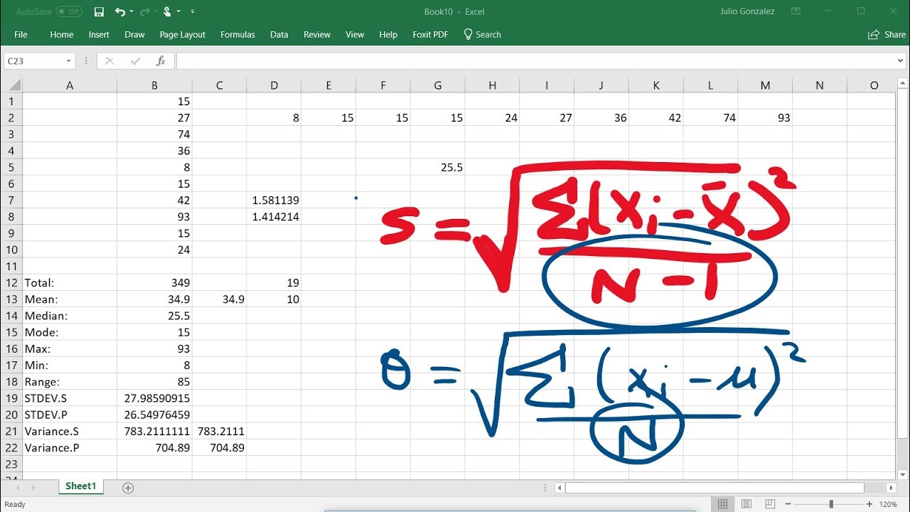
-Variance is a measure that represents the average of the squared deviations from the mean. It is used to quantify the dispersion of a set of data points. The standard deviation is the square root of the variance and provides a measure of spread with the same unit of measure as the original data, making it easier to interpret.
Outlines
📚 Introduction to Descriptive Statistics
The video begins by introducing the topic of descriptive statistics, focusing on how to describe data distributions using meaningful values. The instructor discusses the transition from illustrating data with histograms to using descriptive statistics to summarize data characteristics. The textbook reference for this chapter is mentioned, along with an example of a frequency table for a college algebra class quiz scores. The discrete nature of the quiz scores and the calculation of relative frequencies are highlighted, leading into the concept of cumulative frequencies and their role in understanding data distribution.
🔢 Describing Data with the Arithmetic Mean
The instructor explains the concept of the arithmetic mean, or average, as a measure of central tendency. The calculation of the mean for a population is demonstrated using the quiz scores dataset, resulting in a mean score of 6.8. The notation for the mean in a population (mu) and a sample (x bar) is discussed, along with the distinction between a statistic and a parameter. The mean's sensitivity to outliers and the concept of resistance in numerical summaries are introduced, with the mean being identified as non-resistant due to its vulnerability to the influence of outliers or skewed data.
📈 Understanding Resistance and the Median
The concept of resistance in numerical summaries is further explored, with the median presented as a resistant measure of central tendency. The median's definition as the middle value of a sorted dataset is explained, along with the process of finding the median in both odd and even numbered datasets. The instructor provides examples to illustrate the calculation of the median and emphasizes its resistance to outliers, making it a reliable measure of central tendency.
📊 Calculating the Median in Practice
The practical application of calculating the median is demonstrated using the large college algebra quiz dataset. The process involves identifying the middle scores for an even number of students and averaging them to find the median score, which is determined to be 7. The closeness of the median to the mean score is noted, highlighting the consistency of these two measures of central tendency in this dataset.
🔧 Utilizing a Calculator for Statistical Analysis
The video script shifts focus to the practical use of calculators for statistical analysis. The process of storing data into a calculator's list is detailed, along with the steps to clear existing data and input new data points accurately. The importance of avoiding data entry errors is emphasized, and the process of editing and storing data in list one (L1) is demonstrated.
📈 Creating Histograms with a Calculator
The instructor explains how to use a calculator to create histograms for data visualization. The steps involve accessing the stat plot feature, selecting the appropriate plot type, and setting up the calculator to graph the histogram using the stored data in list one (L1). The use of the zoom feature to size the graph appropriately for the data is also covered, along with troubleshooting tips for clearing any existing functions that might interfere with the histogram display.
📊 Analyzing Data with One Variable Stats
The video concludes with a demonstration of using the calculator to generate a package of statistical summaries for a dataset, referred to as one variable stats. The process includes accessing the calculate menu, selecting the one variable stats option, and inputting the correct list reference. The output provided by the calculator, such as the mean, sum, and other statistical measures, is discussed, showcasing the efficiency of using technology for statistical analysis.
📝 Setting Up the Calculator for Statistics
The final part of the script discusses the setup of the calculator for the semester, including turning off the stat wizards for consistency with textbook screenshots and older calculator models. The difference between the calculator interface with and without stat wizards is explained, and the instructor's preference for operating without them is stated. The importance of this setup in ensuring that all students can follow along with the calculator demonstrations is highlighted.
🏆 Exploring the Mode and Measures of Dispersion
The script introduces the mode as the third measure of central tendency, which is the most frequent observation in a dataset. The potential for a dataset to have no mode, one mode, or multiple modes is discussed, along with the mode's resistance to outliers. The primary use of the mode with categorical variables is explained, as well as its role in contexts like elections. The need for measures of dispersion to complement measures of central tendency is emphasized, with examples of how different datasets can have the same mean and median but different spreads, highlighting the importance of range as a simple measure of dispersion.
📏 Introducing Range and Standard Deviation
The range as a measure of dispersion is defined as the difference between the maximum and minimum values in a dataset. Its sensitivity to outliers is noted, and its limitations as a measure of dispersion are discussed. The standard deviation is introduced as a more informative measure of dispersion, which describes the average spread of data values from the mean. The process of calculating the standard deviation involves first calculating the variance, which is the average of squared deviations from the mean, and then taking the square root of the variance to obtain the standard deviation with the same unit of measure as the original data.
Mindmap
Keywords
💡Descriptive Statistics
💡Frequency Table
💡Histogram
💡Arithmetic Mean
💡Median
💡Cumulative Frequencies
💡Outliers
💡Resistance
💡Mode
💡Range
💡Standard Deviation
Highlights
Introduction to Descriptive Statistics and the concept of describing data distributions.
Explanation of frequency tables and their role in understanding data sets.
Discussion on discrete variables and the example of scores from a college algebra class quiz.
Calculation and interpretation of relative frequencies from the quiz scores.
Introduction of cumulative frequencies and cumulative relative frequencies for data analysis.
The significance of the mean as a measure of central tendency in data sets.
Calculation of the arithmetic mean for the quiz scores and its interpretation.
Difference between population mean (parameter) and sample mean (statistic).
The issue of mean being affected by outliers and the concept of resistance in statistical summaries.
Introduction to the median as a resistant measure of central tendency.
Process of finding the median in both odd and even sized data sets.
Comparison between the mean and median in the context of the college algebra quiz data.
Demonstration of using a calculator for statistical analysis, including storing data in lists.
Building histograms using calculator to visualize data distribution.
Utilization of the calculator to compute one-variable statistics for a data set.
Introduction to the mode as a measure of central tendency and its resistance to outliers.
Importance of measures of dispersion in describing the spread of data sets.
Explanation of range as a simple measure of dispersion and its sensitivity to outliers.
Introduction to variance and standard deviation as measures of spread.
Process of calculating variance and standard deviation by hand for a small data set.
The significance of standard deviation in reflecting the average spread from the mean.
Transcripts
Browse More Related Video
Descriptive Statistics: FULL Tutorial - Mean, Median, Mode, Variance & SD (With Examples)

Elementary Stats Lesson #4
Calculating The Standard Deviation, Mean, Median, Mode, Range, & Variance Using Excel

Introduction to Descriptive Statistics
Descriptive Statistics [Simply explained]

Measures of Variability (Range, Standard Deviation, Variance)
5.0 / 5 (0 votes)
Thanks for rating: