Test of Independence Using Chi-Square Distribution
TLDRThe script analyzes whether the average number of hours high school students spend studying is independent of their grade level. It steps through constructing a contingency table showing the observed data, determining the expected values to test for independence, formulating the null and alternative hypotheses, calculating degrees of freedom, finding the critical value from a chi-square distribution table, computing the test statistic, and comparing it to the critical value in order to make a decision. Since the test statistic falls in the rejection region, there is evidence to reject the null hypothesis and conclude that study time depends on student type, specifically that seniors study less than freshmen.
Takeaways
- 😀 The transcript discusses a statistical analysis using a chi-square test to determine if the average number of study hours is dependent on the type of high school student.
- 📊 A contingency table is constructed showing the number of freshman and senior students studying different hourly ranges.
- 🤔 The null hypothesis is that study hours are independent of student type.
- 📐 Degrees of freedom are calculated to be 2 for the analysis.
- 🔢 Expected values are computed for the contingency table cells.
- ☑️ The calculated chi-square statistic is compared to the critical value.
- ❗ The calculated value falls in the rejection region, so the null hypothesis is rejected.
- 👩🎓 There is evidence that seniors spend less time studying than freshmen.
- 😟 This could be indicative of "senioritis" among the senior students.
- 📋 The analysis demonstrates using chi-square tests for independence with contingency tables.
Q & A
What are the two hypotheses being tested in this analysis?
-The null hypothesis is that the average number of hours studied is independent of the type of student. The alternative hypothesis is that the average number of hours studied depends on the type of student.
How many degrees of freedom are there for the chi-square test?
-There are 2 degrees of freedom, calculated as (number of rows - 1) x (number of columns - 1) = (2-1) x (3-1) = 1 x 2 = 2.
What is the critical value for the chi-square test?
-With 2 degrees of freedom and α = 0.05, the critical chi-square value is 5.99.
What is the calculated chi-square statistic?
-The calculated chi-square statistic is 32.3.
What can we conclude from the chi-square test result?
-Since the calculated chi-square value of 32.3 is greater than the critical value of 5.99, we reject the null hypothesis. There is evidence that the average number of hours studied depends on the type of student.
Which group studies the most hours per day on average?
-Freshmen study the most hours per day on average. The data shows freshmen study 2-4 hours per day more frequently than seniors.
How are the expected frequencies calculated?
-The expected frequencies are calculated by taking the row total × column total / total n. For example, the expected frequency for freshmen studying 2-4 hours is 310 × 252 / 630 = 124.
What assumptions need to be met to use the chi-square test?
-The chi-square test requires that the expected frequencies should be greater than 5 in at least 80% of the cells, and no cell should have an expected frequency of less than 1.
What causes the senioritis mentioned at the end of the transcript?
-Senioritis refers to a decrease in motivation that some students experience their senior year of high school as they look ahead to graduating and moving on from high school.
What additional data could help explain the difference in study hours between freshmen and seniors?
-Data on the difficulty or workload of classes, involvement in extracurricular activities, job/family responsibilities, plans after graduation, and overall motivation levels could help further explain the difference in study hours.
Outlines
📊 Building a Contingency Table for a Chi-Square Test
This paragraph discusses creating a contingency table to perform a chi-square test of independence to determine if the average number of study hours depends on the type of high school student. It calculates the totals for the rows and columns in the table, states the null and alternative hypotheses, calculates the degrees of freedom, and explains the test procedure using the chi-square distribution.
📉 Calculating Expected Values for the Chi-Square Test
This paragraph shows the calculation of the expected values for each cell in the contingency table using the provided formula. It calculates and rounds the expected values and verifies the row and column totals match the original table.
📈 Calculating and Interpreting the Chi-Square Statistic
This paragraph calculates the chi-square statistic using the observed and expected values. It compares the calculated value to the critical value, determines the result falls in the rejection region, rejects the null hypothesis, and concludes there is evidence that average study hours depends on student type, noting seniors spend less time.
Mindmap
Keywords
💡Contingency Table
💡Chi-Square Test of Independence
💡Null Hypothesis
💡Alternative Hypothesis
💡Degrees of Freedom
💡Critical Value
💡Expected Values
💡Calculated Chi-Square Value
💡Rejection Region
💡Significance Level (Alpha)
Highlights
Completes a contingency table to analyze the average number of hours students spend studying
States the null and alternative hypotheses for testing if study hours depends on student type
Calculates 2 degrees of freedom for the chi-square test
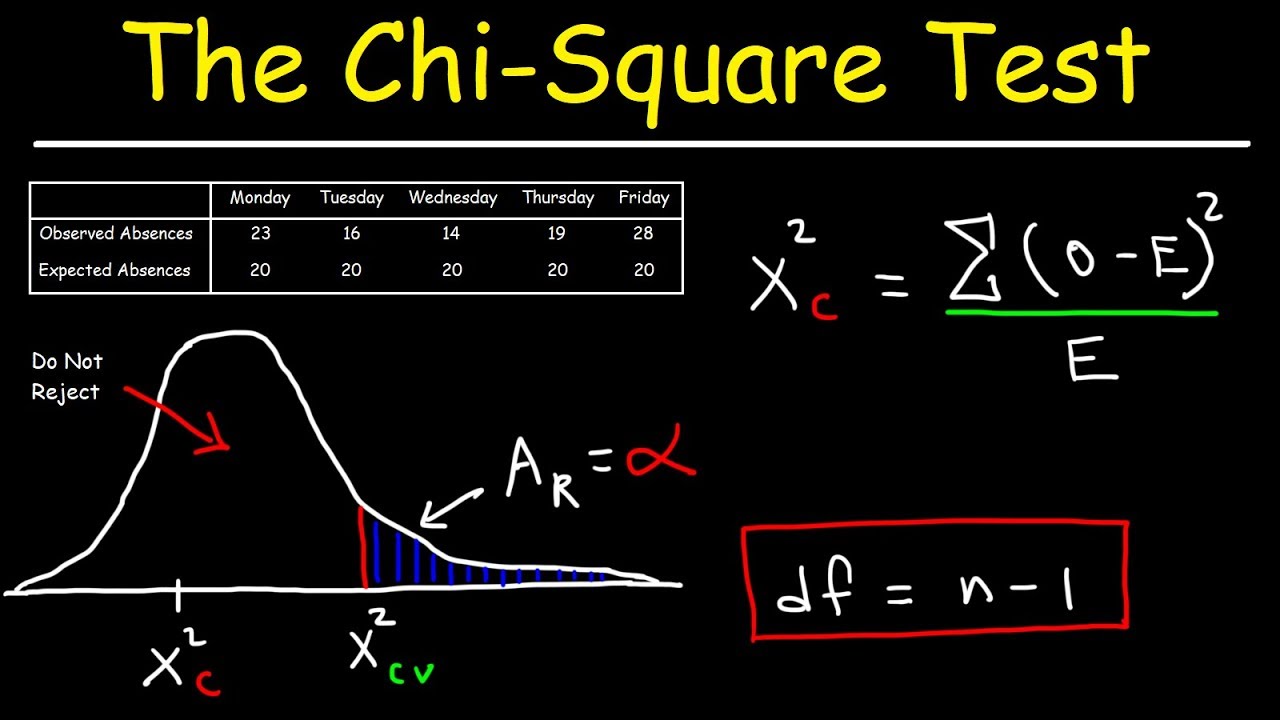
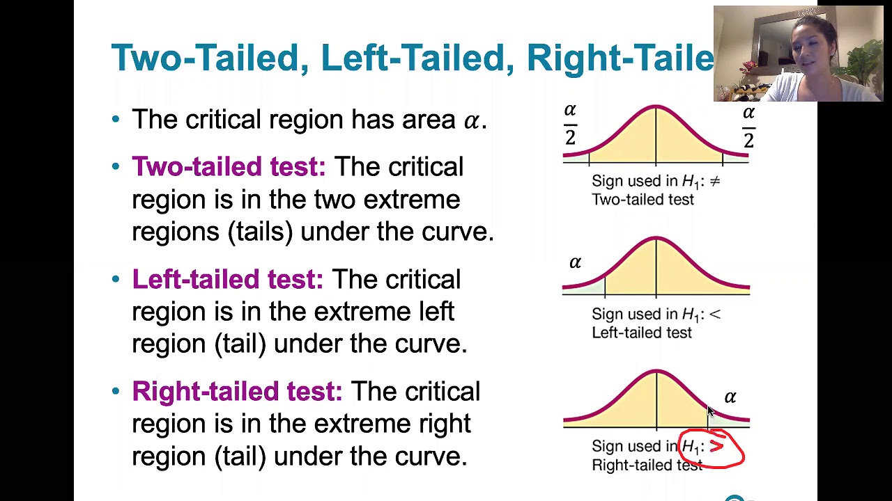
Explains using a right-tailed chi-square test with α = 0.05 significance level
Determines critical chi-square value from table is 5.99 with 2 degrees of freedom
Calculates expected values for each cell in contingency table
Sums differences between observed and expected values squared over expected values to get chi-square statistic
Obtains chi-square test statistic value of 32.3
Compares test statistic to critical value and rejects null hypothesis since it falls in rejection region
Concludes there is evidence that average study hours depends on student type
Seniors spend much less time studying than freshmen
Perhaps seniors have "senioritis" with less motivation to study
Contingency table analysis using chi-square test of independence
Right-tailed test critical region reflects α = 0.05 significance level
Test statistic outside critical value region leads to null hypothesis rejection
Transcripts
Browse More Related Video
5.0 / 5 (0 votes)
Thanks for rating: