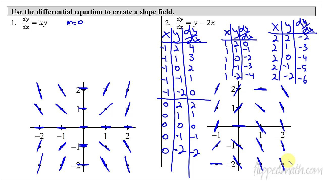
Matching Slope Fields to Differential Equations Part 1
TLDRThe video script discusses the challenging task of matching differential equations to slope fields, a concept that can be daunting for many. The speaker plans to tackle multiple examples, which may result in a lengthy video but promises to be worthwhile. To aid understanding, a PDF with all the equations and concepts discussed will be provided. The process involves analyzing slope fields and systematically eliminating differential equations that don't match the observed characteristics, such as the presence of constant slopes or the influence of x and y variables. The speaker uses visual cues like vertical and horizontal lines and the behavior of the slope field to narrow down the possible equations. Techniques like sketching solution curves and substituting values are employed to match the equations to the correct slope field. The summary of the process demonstrates the systematic approach to solving differential equations, making it engaging for viewers interested in mathematics or those looking to improve their problem-solving skills in this area.
Takeaways
- 📐 **Matching DEs to Slope Fields**: The video discusses how to match differential equations (DEs) to their corresponding slope fields, which can be a challenging task for many people.
- 📚 **PDF Resource**: A PDF with all the DEs and slope fields used in the video is provided, allowing viewers to follow along and try the problems before watching the video.
- 🔍 **Analyzing Slope Fields**: The presenter uses vertical and horizontal line analysis to determine which DE matches a given slope field by observing how the slope changes with X and Y.
- ✅ **Elimination Method**: The process involves eliminating DEs that do not fit the observed behavior of the slope field, such as those that do not contain the correct variables (X or Y).
- 🌊 **Visualizing Solution Curves**: The presenter suggests visualizing the solution curve as a river, dropping a twig into it, and following its path to get a sense of the solution's shape.
- 🔄 **Periodicity Consideration**: When DEs involve trigonometric functions, the period of the function is considered to match the observed pattern in the slope field.
- 🚫 **Zero Slopes**: The presence of zero slopes in the slope field is a key feature to focus on, as it helps narrow down the DEs that could produce such behavior.
- 🔢 **Substitution Method**: Substituting specific values (like Y = -2x) into the remaining DEs helps to further eliminate options and find the correct match.
- 📉 **Slope Sign Analysis**: Observing the sign of the slope in different quadrants can also be used to determine the correct DE, as it provides information about the relationship between X, Y, and dy/dx.
- ⏩ **Efficiency in Process**: As the presenter becomes more familiar with the process, the speed at which DEs are matched to slope fields increases.
- 📺 **Continued in Next Videos**: The video series will continue in subsequent installments to cover more examples of matching DEs to slope fields.
Q & A
What is the main topic of the video?
-The main topic of the video is matching differential equations to slope fields, which is a challenging concept for many people.
Why does the presenter suggest getting a PDF of the problems worked on?
-The presenter suggests getting a PDF so that viewers can try the problems ahead of time and then watch the video for a more effective learning experience.
How does the presenter begin to match the first differential equation to a slope field?
-The presenter begins by analyzing the slope field along vertical lines, noting that the slope is constant, which indicates that the differential equation should only contain 'X'.
What is the presenter's method for visualizing a solution curve?
-The presenter visualizes a solution curve by imagining it as a river and mentally dropping a twig into it, following the path that the twig would take.
How does the presenter determine the period of the function for the first differential equation?
-The presenter estimates the distance between the peaks of the sine function in the slope field to be roughly PI, which indicates a period of PI, helping to choose the correct differential equation.
What is the significance of looking for zero slopes in the slope field?
-Zero slopes are significant because they indicate points where the differential equation equals zero, which can help in identifying the correct equation.
How does the presenter use the line y equals negative 2x in the second differential equation?
-The presenter substitutes Y with negative 2x in the remaining differential equations to see which one simplifies to zero, as the slopes along y equals negative 2x should be zero.
What is the strategy for the third differential equation?
-The presenter draws a strategic vertical line at x equals 0 and observes that the slopes are zero along this line, which helps to eliminate differential equations that do not result in zero slopes.
Why does the presenter focus on quadrant one for the third differential equation?
-The presenter focuses on quadrant one because in this quadrant both x and y are positive, but dy/dx is negative, which is a condition that only one of the remaining differential equations can satisfy.
What is the presenter's approach to making the process quicker as more differential equations are solved?
-The presenter's approach is to apply the insights gained from solving previous equations to quickly eliminate incorrect options and focus on the most likely correct equations.
Why does the presenter decide to split the video into multiple parts?
-The presenter decides to split the video into multiple parts due to the length of the first part and the complexity of the topic, ensuring that the information is digestible and viewers can follow along effectively.
What does the presenter wish for the viewers at the end of the video?
-The presenter wishes the viewers good luck and encourages them to come back for the next video in the series for further learning.
Outlines
📚 Introduction to Matching Differential Equations to Slope Fields
The speaker introduces the topic of the video, which is about matching differential equations to slope fields, a concept that many find challenging. They mention that they will be discussing many examples, which might make the video lengthy, but ultimately informative. The speaker also provides a PDF link for viewers to follow along and suggests that viewers might want to try the problems before watching the video. The video starts with a set of 16 differential equations that will be matched to slope fields, which include various types such as those involving X, Y, or trigonometric functions. The first step is to analyze a slope field and determine which differential equation it corresponds to by looking at vertical and horizontal lines and deducing that the slope is not influenced by the value of Y, thus narrowing down the options to those without Y.
🔍 Analyzing Slope Fields and Differential Equations
The speaker continues by discussing the process of elimination when matching differential equations to a given slope field. They illustrate this by drawing vertical and horizontal lines on the slope field and observing how the slope changes with X and Y. The goal is to identify which parts of the equation (X, Y, or both) are influencing the slope. The speaker then focuses on zero slopes, which are important to highlight, and sketches a line where the slope is zero. By substituting Y with -2X in the remaining differential equations, they are able to further narrow down the options. The process involves simplifying the equations and checking which one results in zero when the conditions of the slope field are met. The video concludes with the speaker identifying the correct differential equation for the second slope field and hints at continuing the discussion in subsequent videos.
Mindmap
Keywords
💡Differential Equations
💡Slope Fields
💡Vertical and Horizontal Lines
💡Solution Curve
💡Trigonometric Functions
💡Derivatives
💡Period
💡Zero Slopes
💡Strategic Vertical Line
💡Substitution
💡Quadrants
Highlights
The video discusses matching differential equations to slope fields, which is a challenging topic for many people.
A PDF of the differential equations discussed in the video is provided for viewers to follow along.
The presenter will work through multiple examples to demonstrate the process of matching.
Different types of differential equations are presented, including those with X, Y, and trigonometric functions.
The method of analyzing slope fields by looking along vertical and horizontal lines is introduced.
The importance of identifying when the slope is constant along a vertical line is emphasized, indicating the differential equation will only contain X.
The presenter demonstrates how to visualize solution curves by imagining a river and following a hypothetical 'tweak'.
The resemblance of the solution curve to y = -cos(X) is used to narrow down the differential equations.
The derivative of -cos(X) is identified as the differential equation, which helps eliminate options that don't match.
The period of the solution curve is considered to further refine the selection of the correct differential equation.
The video shows how to eliminate differential equations that do not account for zero slopes observed in the slope field.
Substituting Y with -2X in the remaining differential equations helps to find the one that results in zero slope.
The presenter identifies a line where the slope is always negative one, which helps in selecting the correct differential equation.
The video demonstrates the process of substituting values into the differential equations to find the one that matches the slope field.
The importance of considering the signs of X and Y in different quadrants to determine the correct differential equation is highlighted.
The presenter plans to create more videos to continue the discussion on matching differential equations to slope fields.
The video concludes with an invitation for viewers to return for the next video in the series.
Transcripts
5.0 / 5 (0 votes)
Thanks for rating:
