Lec 1 | MIT 18.03 Differential Equations, Spring 2006
TLDRThe video script is a detailed lecture on differential equations, focusing on first-order ordinary differential equations (ODEs). The lecturer assumes the audience has a basic understanding of ODEs and modeling, and thus, delves into the specifics of first-order ODEs. The script explains the standard form of these equations and introduces the concept of solving them through separation of variables, although it acknowledges that not all such equations are solvable using this method. The lecture emphasizes the geometric interpretation of differential equations using direction fields and integral curves, contrasting this with the analytic method of solving them. The direction field is portrayed as a visual representation where each point on the field has a specific slope determined by the differential equation, and the integral curves are the solutions to the ODEs, graphically represented as curves tangent to the direction field at every point. The script guides through the process of plotting direction fields and integral curves, highlighting the efficiency of plotting isoclines (lines of constant slope) before drawing line elements. It also discusses the limitations of solutions' domains and the challenges in predicting them without explicit calculation or computer visualization. The lecturer further illustrates the process with examples, including an ODE representing motion where the solution curves are circles, and another example where the integral curves cannot cross or touch each other due to the Existence and Uniqueness Theorem. This theorem guarantees that for a given point, there is exactly one solution to the differential equation, provided certain conditions are met, such as the function being continuous with a continuous partial derivative. The script concludes with a practical example of solving an ODE by separation of variables and plotting the solutions, emphasizing the importance of understanding the domain of solutions and the conditions under which the Existence and Uniqueness Theorem applies.
Takeaways
- 📚 Start with the assumption that students have prior knowledge of differential equations and modeling from high school or 18.01 course.
- 🔢 Focus on first-order ordinary differential equations (ODEs), which are written in standard form with the derivative isolated on one side.
- 📈 Understand the difference between solvable and unsolvable ODEs; some equations look simple but have no elementary function solutions.
- 📈📉 The geometric view of differential equations involves direction fields and integral curves, contrasting with the analytic method that seeks explicit solutions.
- 🌐 Direction fields are represented on a plane with line elements (or vector fields) indicating the slope of the solution at each point.
- 🔍 Isoclines are curves on the plane where the slope of the line element is constant; they are useful for sketching direction fields by hand.
- ➗ The x-axis and y-axis can be considered as special isoclines representing infinite and zero slopes, respectively.
- 🚫 Integral curves, representing solutions, cannot cross each other at an angle or touch, due to the uniqueness of the slope at any given point.
- 🔑 The Existence and Uniqueness Theorem guarantees that through a given point, there is exactly one solution to the differential equation, provided certain conditions are met.
- 📈 For some differential equations, solutions can be found by separation of variables, which can also provide insight into the behavior of solutions.
- 📊 The domain of a solution may be limited and is not always obvious from the differential equation alone; it may require explicit calculation or graphical analysis.
- 💻 Numerical methods and computer simulations can be used to approximate solutions and visualize the behavior of solutions when analytic solutions are not available or are complex.
Q & A
What is the main topic of the lecture?
-The main topic of the lecture is the exploration of first-order ordinary differential equations (ODEs), focusing on their geometric interpretation and numerical solutions, rather than just the analytic method.
What is the standard form of a first-order ODE?
-The standard form of a first-order ODE is where the derivative of y with respect to x is isolated on the left-hand side, and everything else is on the right-hand side.
What is an integral curve in the context of differential equations?
-An integral curve is a curve that passes through the plane at every point tangent to the line element of the direction field associated with the differential equation.
What is a direction field?
-A direction field is a graphical representation where each point in the plane is associated with a line element (or vector) that has a slope corresponding to the value of the derivative at that point according to the differential equation.
How does the lecturer suggest drawing a direction field by hand?
-The lecturer suggests starting by plotting isoclines, which are curves where the slope of the line element is a constant value (C), and then drawing line elements with the corresponding slopes.
What is an isocline?
-An isocline is a curve on the plane where the slope of the line element is a constant value (C). It is used to help plot the direction field when solving differential equations geometrically.
Why can't two integral curves cross each other at an angle?
-Two integral curves cannot cross each other at an angle because at the point of intersection, there would be ambiguity in the slope of the direction field, as each curve would impose a different slope, which is not allowed.
What is the significance of the Existence and Uniqueness Theorem in the context of differential equations?
-The Existence and Uniqueness Theorem guarantees that for a given initial condition, there is exactly one solution to the differential equation that passes through that point, provided certain conditions (like continuity of the function and its partial derivatives) are met.
Why might the Existence and Uniqueness Theorem not apply to a certain point?
-The Existence and Uniqueness Theorem might not apply if the function f(x, y) is not continuous or its partial derivative with respect to y is not continuous near the point in question.
What is Euler's method, and how does it relate to the lecture?
-Euler's method is a numerical technique used to approximate solutions of differential equations. It is mentioned in the lecture as a topic for self-study, as the lecturer chooses to focus on geometric and numerical approaches to understanding differential equations.
How does the lecturer illustrate the concept of limited domains for solutions of differential equations?
-The lecturer uses the example of solutions represented as circles with centers at the origin, explaining that the domain of these solutions is limited to a certain range of x-values and cannot be extended further without violating the properties of the solution.
Outlines
😀 Introduction to First-Order ODEs
The speaker begins by assuming the audience has a basic understanding of differential equations and modeling from previous education. They will not be explaining what differential equations or modeling are, but will focus on first-order ordinary differential equations (ODEs). The standard form of these ODEs is discussed, along with examples. The concepts of solvability and the difference between solvable and unsolvable equations in the context of elementary functions are introduced. The lecture aims to address how to approach unsolvable equations and introduces the idea of looking at differential equations geometrically and numerically.
📐 Analytic vs. Geometric Views of ODEs
The paragraph explains the difference between the analytic method of solving ODEs, which involves finding explicit functions that satisfy the equation, and the geometric view, which involves direction fields and integral curves. A direction field is a visual representation where each point on the plane has a line element with a slope corresponding to the differential equation. An integral curve is a curve that at every point is tangent to the corresponding line element in the direction field. The relationship between the graph of a solution and the integral curve is established, and it is shown that drawing an integral curve geometrically is equivalent to solving the ODE analytically.
🤖 Computer-Generated Direction Fields
The speaker discusses how computers generate direction fields by calculating the function value at each point on a grid and then drawing line elements with the corresponding slope. The spacing of points and the length of the line elements can be adjusted, and the process is considered naive due to the straightforward computation at each point. The human approach to drawing direction fields is contrasted, emphasizing the importance of understanding the concept rather than just following a mechanical process.
🧐 Human Approach to Direction Fields
The human method for drawing direction fields is described as more intelligent and efficient. Instead of starting with points, one begins with a desired slope (C) and plots the corresponding isocline, which is a curve where the slope is constant. The isoclines are drawn using dashed lines to distinguish them from the integral curves (solutions), which are drawn with solid lines. The process is demonstrated with examples, showing how to fill the plane with line elements of a specific slope to form the direction field.
🔄 Isoclines and Integral Curves for Specific ODEs
The paragraph delves into finding isoclines and drawing integral curves for a given differential equation (y prime equals minus x over y). The isoclines are lines through the origin, and the integral curves are shown to be circles with centers at the origin. The solutions to the ODE are expressed in terms of square roots and are limited in domain, which is a common challenge when dealing with differential equations. The importance of understanding the domain of a solution is emphasized.
🚫 Principles of Integral Curves
The speaker outlines two key principles regarding integral curves. First, no two integral curves can cross each other at an angle because this would imply two different slopes at the same point, which is not allowed by the direction field. Second, integral curves cannot even touch, let alone cross, each other. This is explained by the Existence and Uniqueness Theorem, which states that for a given point, there is exactly one solution to the differential equation. The theorem's hypotheses are also discussed, including the need for the function and its partial derivative with respect to y to be continuous.
📈 Existence, Uniqueness, and Euler's Method
The final paragraph discusses the application of the Existence and Uniqueness Theorem to a specific differential equation. It is shown that the theorem does not apply along the y-axis where the function is not defined, leading to a failure of uniqueness. The example demonstrates that the theorem must be applied carefully, ensuring that the differential equation is in the proper form and that the function meets the required conditions. The speaker also mentions Euler's method but decides to forgo a detailed explanation, instead choosing to provide an example to solidify the concepts discussed.
Mindmap
Keywords
💡Differential Equations
💡First-Order ODEs
💡Separation of Variables
💡Direction Field
💡Integral Curve
💡Isoclines
💡Existence and Uniqueness Theorem
💡Euler's Method
💡Geometric View
💡Analytic Method
💡Numerical Solutions
Highlights
Introduction to first-order ordinary differential equations (ODEs) and their standard form.
Assumption that students are familiar with basic concepts of ODEs and modeling from prior education.
Explanation of the difference between solvable and unsolvable ODEs, even when they appear similar.
Introduction to the geometric view of differential equations as an alternative to the analytic method.
Definition and explanation of a direction field and its relation to the differential equation.
Description of an integral curve as a curve that is everywhere tangent to the direction field.
Theorem stating that a function is a solution to an ODE if and only if its graph is an integral curve of the associated direction field.
Technique for drawing direction fields using computers versus the more intelligent human approach.
Process of plotting isoclines to draw direction fields and the concept of using slope values to determine them.
Example of drawing a direction field for the ODE y' = -x/y, including the calculation of isoclines and integral curves.
Discussion on the limited domain of solutions for certain ODEs and the challenges in determining this domain.
Second example using the ODE y' = 1 + x - y, demonstrating the process of drawing a direction field and predicting behavior of solutions.
Principle that two integral curves cannot cross at an angle and the implications for drawing direction fields.
Existence and Uniqueness Theorem and its importance in ensuring that through a given point, there is exactly one solution to an ODE.
Conditions under which the Existence and Uniqueness Theorem applies, including the continuity of the function and its partial derivative.
Illustration of the theorem's failure and the importance of the differential equation being in standard form for the theorem to hold.
Practical implications of the Existence and Uniqueness Theorem in real-world applications of differential equations.
Brief mention of Euler's method and its application in solving differential equations numerically.
Transcripts
Browse More Related Video

The Geometric Meaning of Differential Equations // Slope Fields, Integral Curves & Isoclines
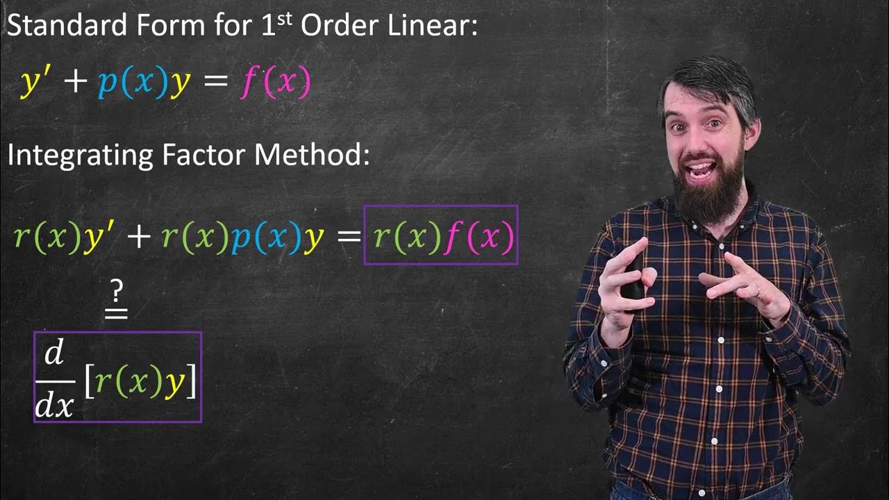
Linear Differential Equations & the Method of Integrating Factors

Ordinary Differential Equations 1 | Introduction
AP Calculus AB: Lesson 7.2 Slope Fields

SC_V1_1 ODE Trick: Separation of Variables (Leibniz Rule)

The Theory of 2nd Order ODEs // Existence & Uniqueness, Superposition, & Linear Independence
5.0 / 5 (0 votes)
Thanks for rating: