Calculus AB/BC – 7.3 Sketching Slope Fields
TLDRThe video script is an educational tutorial featuring Mr. Bean, who guides viewers on how to sketch a slope field, a graphical representation of the slope of every possible solution to a differential equation. He uses the example of dy/dx = 2x to illustrate how to determine the slope at specific points and introduces the concept of the general solution, denoted by 'plus c'. Mr. Bean also demonstrates the use of a GeoGebra app to visualize slope fields and plot solution curves for a better understanding of the underlying differential equations. The tutorial emphasizes the importance of accurately plotting hash marks for slopes of zero and provides strategies for sketching slope fields, including focusing on points with zero slopes and using a chart for systematic calculations. The script concludes with an exercise for the audience to practice sketching a slope field and hints at future lessons that will delve deeper into solving differential equations and graphing solutions.
Takeaways
- 📈 A slope field is a graphical representation of the slopes of the solutions to a differential equation at every point in the xy-plane.
- 🔍 The slope at any given point on the field can be found by plugging the x and y coordinates into the differential equation.
- 🌟 The general solution to a differential equation can be represented by adding a constant (C) to the antiderivative of the equation.
- 📊 GeoGebra is a useful tool for visualizing slope fields and plotting solutions to differential equations.
- 🎨 When sketching a slope field by hand, it's helpful to start with points where the slope is zero, such as where x or y equals zero.
- 👀 Eyeballing is a common technique for approximating the slope of a tangent line at a given point when exact calculation isn't feasible.
- 🔢 It's important to ensure that horizontal and vertical lines (where the slope is zero or undefined) are accurately represented in the slope field.
- 📐 The process of graphing a slope field involves plotting hash marks at each point to indicate the slope, creating a visual current that represents the direction of the solution curves.
- 🔍 To find a particular solution, one can select a point and follow the 'current' of the slope field to trace out the solution curve.
- 🔑 Identifying key features like horizontal and vertical hash marks can help in determining the differential equation from a given slope field.
- 🧮 Sometimes, creating a table of values for different x and y coordinates can assist in calculating the slopes and sketching the slope field more systematically.
Q & A
What is a slope field?
-A slope field is a graphical representation of a differential equation. It shows the slope of every possible solution to the differential equation at every point in the field.
How does a slope field help in understanding differential equations?
-A slope field provides a visual representation of the solutions to a differential equation. It shows the direction and steepness of the slope at each point, which can help in visualizing the shape of the actual solution curves.
What is the differential equation used as an example in the script?
-The differential equation used as an example is dy/dx = 2x.
How can you find the slope at a specific point in a slope field?
-To find the slope at a specific point, you substitute the x and y coordinates of that point into the differential equation. The result gives you the slope at that point.
What is the general solution to the example differential equation dy/dx = 2x?
-The general solution to the differential equation dy/dx = 2x is y = x^2 + C, where C is the constant of integration.
How can you use a tool like GeoGebra to explore slope fields?
-GeoGebra can be used to plot slope fields for various differential equations. By entering the differential equation into the tool, you can see the slope field and even plot solution curves by selecting different values for the constant of integration.
What is the significance of horizontal hash marks in a slope field?
-Horizontal hash marks in a slope field represent points where the slope is zero. This typically occurs when the x or y value is zero, indicating a flat tangent line at those points.
How can one sketch a slope field by hand?
-To sketch a slope field by hand, one can start by identifying points with a slope of zero, then move on to other points and calculate the slope using the differential equation. The slopes are then represented by hash marks on the graph, with the direction of the hash mark indicating the direction of the slope.
Why is it useful to create a chart when sketching a slope field?
-Creating a chart helps to organize the calculations for different points in the slope field. It allows you to systematically plug in x and y values, calculate the slopes, and keep track of the results, which can be especially helpful for complex differential equations.
What does the script suggest for visualizing the hash marks in a slope field?
-The script suggests visualizing the hash marks as a current on a river. The current pushes a leaf (representing a solution curve) in different directions, giving a sense of the flow and direction of the solution curves.
How can you find the equation of a tangent line at a specific point on a slope field?
-To find the equation of a tangent line, you substitute the x and y coordinates of the specific point into the differential equation to find the slope at that point. Then, using the point-slope form of a line equation, you can write the equation of the tangent line.
Outlines
📊 Introduction to Slope Fields and Differential Equations
Mr. Bean explains the concept of slope fields, which graphically represent differential equations by showing tiny hash marks indicating slopes at various points. Using a specific example of the differential equation dy/dx = 2x, he illustrates how to plot slope points based on input coordinates, emphasizing how these slope fields visually represent all potential solutions to the equation by varying the constant 'C'. He introduces a practical application using the GeoGebra tool to plot these slope fields and visualize how altering 'C' affects the slope of the parabola represented by the equation y = x^2 + C.
🔍 Detailed Analysis of Slope Fields Using GeoGebra
Continuing from the introduction, Mr. Bean uses the GeoGebra tool to show more detailed slope fields by adjusting the density of hash marks, helping visualize the graph's behavior better. He likens the directional flow of the hash marks to the current of a river influencing a leaf's path. A practical exercise is introduced where viewers are encouraged to plot their own slope fields using provided coordinates and compare them against Mr. Bean’s example, promoting interactive learning. He fixes a previous mistake in the slope calculations live, highlighting the real-world challenge of accurately graphing steep slopes.
🧮 Applying Concepts to Predict Graph Behavior and Equation Derivation
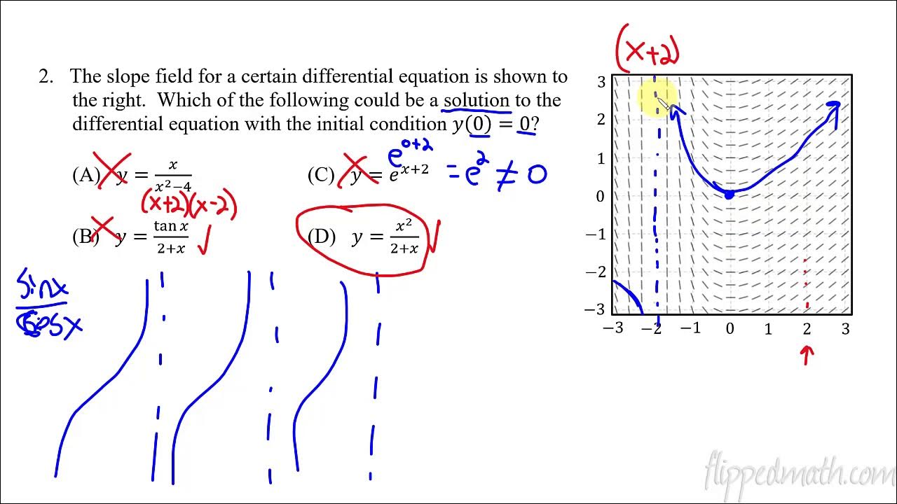
Mr. Bean demonstrates how to use slope fields to predict the behavior of graphs and derive equations of tangent lines at specific points using the slope field and differential equations. He provides a practical application of these concepts with the GeoGebra tool, enhancing the understanding by visualizing how these tangent lines integrate into the graph. The lesson concludes with an exercise to match slope fields with potential equations by identifying key characteristics like horizontal and vertical hash marks and testing points against proposed equations, fostering a deeper comprehension of differential equations.
Mindmap
Keywords
💡Slope Field
💡Differential Equation
💡Anti-Derivative
💡GeoGebra
💡General Solution
💡Tangent Line
💡Point-Slope Form
💡Slope
💡Hash Marks
💡Derivative
💡Graph
Highlights
Mr. Bean introduces the concept of a slope field, which is a graph representing the slope of every possible solution to a differential equation.
Slope fields show tiny hash marks that represent the slope at a particular point on the graph.
An example is given where the differential equation dy/dx = 2x is used to illustrate how to determine the slope at a chosen point, such as (-1, 1).
The anti-derivative of the differential equation is taken to find the general solution, which is y = x^2 + C.
GeoGebra is used to visualize slope fields and allows users to input any differential equation to see the resulting slope field.
The slope field can represent any possible value of C, showing a range of solutions rather than just one.
A method for sketching slope fields is demonstrated, focusing on the slope at specific points rather than exact solutions.
Hash marks for slope fields are drawn for points where x or y equals zero, indicating a slope of zero.
The process of eyeballing the slope and drawing hash marks for each point on the grid is explained.
A chart is suggested for keeping track of slopes at different points, which can be helpful for more complex slope fields.
The importance of accurately plotting horizontal and vertical hash marks is emphasized for understanding the graph's behavior.
The slope field provides a visual representation of the graph's behavior, offering insight into the general solution's shape.
The analogy of a river current is used to describe how the slope field's hash marks can guide the direction of a solution path.
The process of finding the equation of a tangent line from a slope field is demonstrated using point-slope form.
GeoGebra is used again to visualize the tangent line and how it matches up with the slope field.
A strategy for working backward from a slope field to find the original differential equation is discussed, focusing on horizontal and vertical hash marks.
The use of a chart to systematically plug in points and test for the correct differential equation is shown.
The lesson concludes with a reminder that the focus is on understanding slope fields and their representation of general solutions, with specific solution graphs to be covered in the next lesson.
Transcripts


5.0 / 5 (0 votes)
Thanks for rating: