AP Calculus AB: Lesson 7.2 Slope Fields
TLDRIn this instructional lesson, Michelle Kremmel introduces the concept of estimating solutions to differential equations using slope fields when algebraic solutions are unattainable. She demonstrates how to graphically approximate solutions by calculating slopes at various points, creating a slope field to visualize the tangent lines of potential solutions. Kremmel also illustrates the process of sketching solution curves that pass through specific points and highlights the difference between autonomous and non-autonomous differential equations. The lesson concludes with finding particular solutions using initial conditions, emphasizing the practical approach to solving complex differential equations.
Takeaways
- 📚 The lesson focuses on estimating solutions to differential equations using slope fields when separation of variables is not possible.
- 🔍 The example given is a differential equation \( \frac{dy}{dx} = x + y \) which cannot have its variables separated, illustrating the need for an alternative method.
- 📈 The concept of a slope field is introduced as a graphical method to estimate solutions by showing the slope of the tangent line to the solution curve at any point.
- 📝 At any point on the curve, the slope can be determined from the differential equation, providing information about the direction and rate of change of the solution.
- 📍 The importance of knowing at least one point on the graph to sketch a solution in the slope field is emphasized, as it provides a starting point for the estimation.
- 🤔 The process of creating a slope field involves calculating slopes at various points and drawing short segments of tangent lines to represent these slopes.
- 📐 The script demonstrates how to sketch a slope field and solution curve for an autonomous differential equation where the slope depends only on x, not y.
- 📉 The video also covers how to handle non-autonomous differential equations where the slope is dependent on both x and y, requiring consideration of both variables when creating the slope field.
- 👀 The instructor shows the process of sketching solution curves by following the direction of the tangent lines in the slope field and making adjustments as new slope marks are encountered.
- 🔢 The lesson includes solving a differential equation to find a particular solution using initial conditions, demonstrating how the graphical estimation aligns with the algebraic solution.
- 🔍 The benefits and limitations of sketching solution curves with widely spaced slope marks versus more densely packed marks are discussed, highlighting the trade-offs between accuracy and ease of visualization.
Q & A
What is the main topic of this lesson?
-The main topic of this lesson is estimating solutions to differential equations using slope fields.
Why can't the differential equation in the example be solved using separation of variables?
-The differential equation d y/d x = x + y cannot be solved using separation of variables because the variables cannot be separated; the y term does not get isolated on one side when attempting to rearrange the equation.
What does the slope field represent in the context of differential equations?
-A slope field is a visual representation of all possible solutions to a given differential equation, showing the slope at any given point on the plane.
How can the slope at a specific point on a curve be determined from the differential equation?
-The slope at a specific point can be determined by substituting the x and y coordinates of that point into the differential equation, which gives the value of the derivative at that point.
What is the significance of knowing the slope of the curve at any point even if the equation of the curve is unknown?
-Knowing the slope of the curve at any point provides information about the direction and rate of change of the function at that point, which can help in estimating the shape and behavior of the graph.
How can tangent lines be used to approximate the graph of y = f(x) in slope fields?
-Tangent lines can be used to approximate the graph of y = f(x) by following the direction of the tangent lines in the slope field, adjusting the direction as new slope marks are encountered, and staying close to the point of tangency.
What is an autonomous differential equation?
-An autonomous differential equation is one where the differential equation is solely expressed in terms of x and not in terms of y, meaning the slope depends only on the x coordinate.
Why is it important to know at least one point on the graph when sketching a solution in a slope field?
-Knowing at least one point on the graph is important because it provides a starting point for sketching the solution curve in the slope field, allowing for an estimation of the graph's path.
How can the efficiency of creating a slope field be improved?
-The efficiency of creating a slope field can be improved by calculating slopes at regular intervals and identifying patterns or specific conditions that result in slopes of zero or other easily recognizable values.
What is the process of finding a particular solution to a differential equation given an initial condition?
-To find a particular solution, one must first derive the general solution of the differential equation, then apply the initial condition to solve for any constants involved, resulting in a particular solution that satisfies the initial condition.
Outlines
📚 Introduction to Estimating Solutions with Slope Fields
In this lesson, Michelle Kremmel introduces the concept of estimating solutions to differential equations using slope fields when separation of variables is not possible. The example given is a differential equation \( \frac{dy}{dx} = x + y \), which cannot be solved using traditional algebraic methods. Instead, graphical estimation is employed by understanding the slope of the tangent line at any point on the curve, derived from the differential equation itself. The process involves calculating the slope at various points and using this information to sketch the solution curve, even without knowing the explicit function \( y = f(x) \).
📐 Understanding and Creating Slope Fields
This paragraph delves into the specifics of creating a slope field for a given differential equation. The example used is \( \frac{dy}{dx} = x - 1 \), which is an autonomous differential equation, meaning the slope is dependent solely on the x-coordinate. The process involves calculating the slope at specific points and drawing the corresponding tangent lines to create the slope field. The slope field serves as a visual representation of possible solutions, guiding the sketching of the solution curve that passes through a given point, such as (-1, 1).
🔍 Sketching Solution Curves and the Role of Initial Conditions
The focus of this paragraph is on the actual sketching of solution curves within the slope field. It emphasizes the importance of knowing at least one point on the function's graph to accurately sketch the solution. The process involves following the direction of the slope field marks and adjusting the curve as new slope marks are encountered. The paragraph also illustrates how different starting points can lead to visually different solution curves, highlighting the iterative nature of sketching within a slope field.
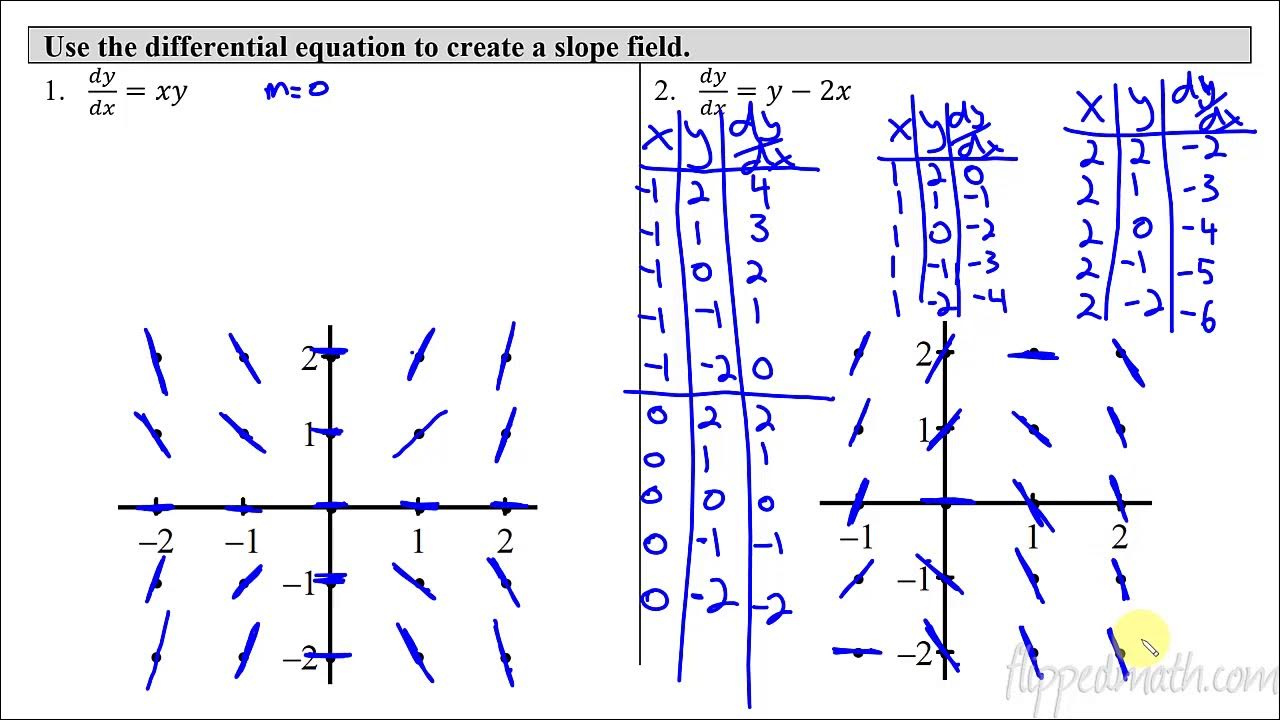
📉 Efficiently Generating a Slope Field for a Non-Autonomous DE
This section discusses the efficient creation of a slope field for a non-autonomous differential equation, \( \frac{dy}{dx} = x - y \). Unlike autonomous equations, the slope here depends on both x and y. The speaker outlines a strategy for identifying points with slopes of zero and one, which are easier to draw, and then moves on to plotting other points systematically. The aim is to fill in the slope field in a way that is not only accurate but also time-efficient.
🤔 Adjusting Sketching Techniques for Sparse Slope Fields
The paragraph discusses the challenges of sketching solution curves when the slope field marks are spaced far apart, resulting in less information for accurate curve drawing. It demonstrates how to adjust the sketching process by using closer tangent lines for a better visualization of the solution curve. The speaker also shows how adjusting the spacing of slope marks can greatly affect the ease of sketching and the accuracy of the resulting curve.
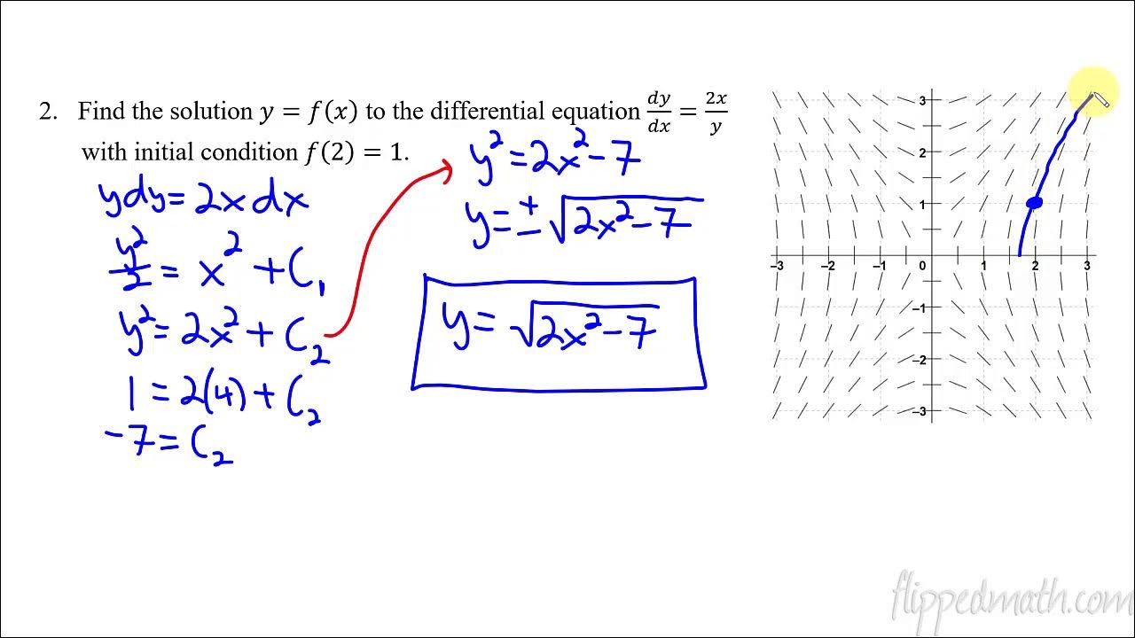
🧩 Completing the Slope Field Sketch with Multiple Examples
In this final paragraph, the speaker wraps up the lesson by providing a comprehensive overview of the process for sketching slope fields and solution curves. Multiple examples are used to illustrate different scenarios, including cases where the slope field is autonomous or not, and where the initial conditions lead to horizontal or vertical tangents. The speaker also solves a differential equation to find a particular solution that matches the sketched curve, reinforcing the connection between graphical estimation and algebraic solution.
Mindmap
Keywords
💡Differential Equation
💡Slope Field
💡Separation of Variables
💡Derivative
💡Tangent Line
💡Autonomous Differential Equation
💡Initial Condition
💡Slant Asymptote
💡Integration
💡Square Root
Highlights
Introduction to estimating solutions to differential equations using slope fields when separation of variables is not applicable.
Demonstration of a differential equation that cannot have variables separated, illustrating the need for alternative solution methods.
Explanation of estimating solutions graphically using slope fields even without knowing the explicit function form.
How to determine the slope of a curve at any point from a given differential equation.
The concept of a slope field as a visual representation of possible solutions to a differential equation.
Technique for sketching a slope field by calculating slopes at specific points in the plane.
The importance of knowing at least one point on the graph to accurately sketch a solution in a slope field.
Efficient method for creating a slope field by identifying patterns and points where the slope is zero or a simple value.
Differentiating between autonomous and non-autonomous differential equations and their impact on slope field construction.
Practical example of sketching a slope field for a differential equation where the slope is solely dependent on the x-coordinate.
How to use the slope field to approximate the graph of y = f(x) by adjusting direction based on nearby slope marks.
The process of finding a particular solution to a differential equation given an initial condition.
Solving a differential equation by integrating both sides and applying initial conditions to find the constant.
Illustration of sketching a solution curve that passes through a specific point using the direction of tangent lines in the slope field.
The impact of slope mark spacing on the accuracy and ease of sketching solution curves within a slope field.
Final example involving a differential equation with a slope dependent on both x and y, and the method to sketch its slope field.
Conclusion summarizing the lesson on slope fields and their application in estimating solutions to differential equations.
Transcripts
Browse More Related Video
AP Calculus BC Lesson 7.5
Calculus AB/BC – 7.3 Sketching Slope Fields
Creating a slope field | First order differential equations | Khan Academy

Lec 1 | MIT 18.03 Differential Equations, Spring 2006

Introduction to Slope Fields (Differential Equations 9)
Calculus AB/BC – 7.7 Particular Solutions using Initial Conditions and Separation of Variables
5.0 / 5 (0 votes)
Thanks for rating: