Average Value of a Function Over an Interval - Calculus
TLDRThe video script discusses the concept of finding the average value of a function over a given interval. It explains the process using three different functions: linear, quadratic, and square root. The script highlights that for a linear function, the average value equals the average y-value, but this relationship varies for non-linear functions. It also introduces the mean value theorem and demonstrates how to calculate the average value and the corresponding x-value (c) where the area under the curve equals the area of the rectangle, using definite integrals and anti-derivatives.
Takeaways
- 📈 The average value of a function over an interval can be found using the definite integral and the Mean Value Theorem.
- 🌟 For a linear function, the average value of the function equals the average y-value on the interval.
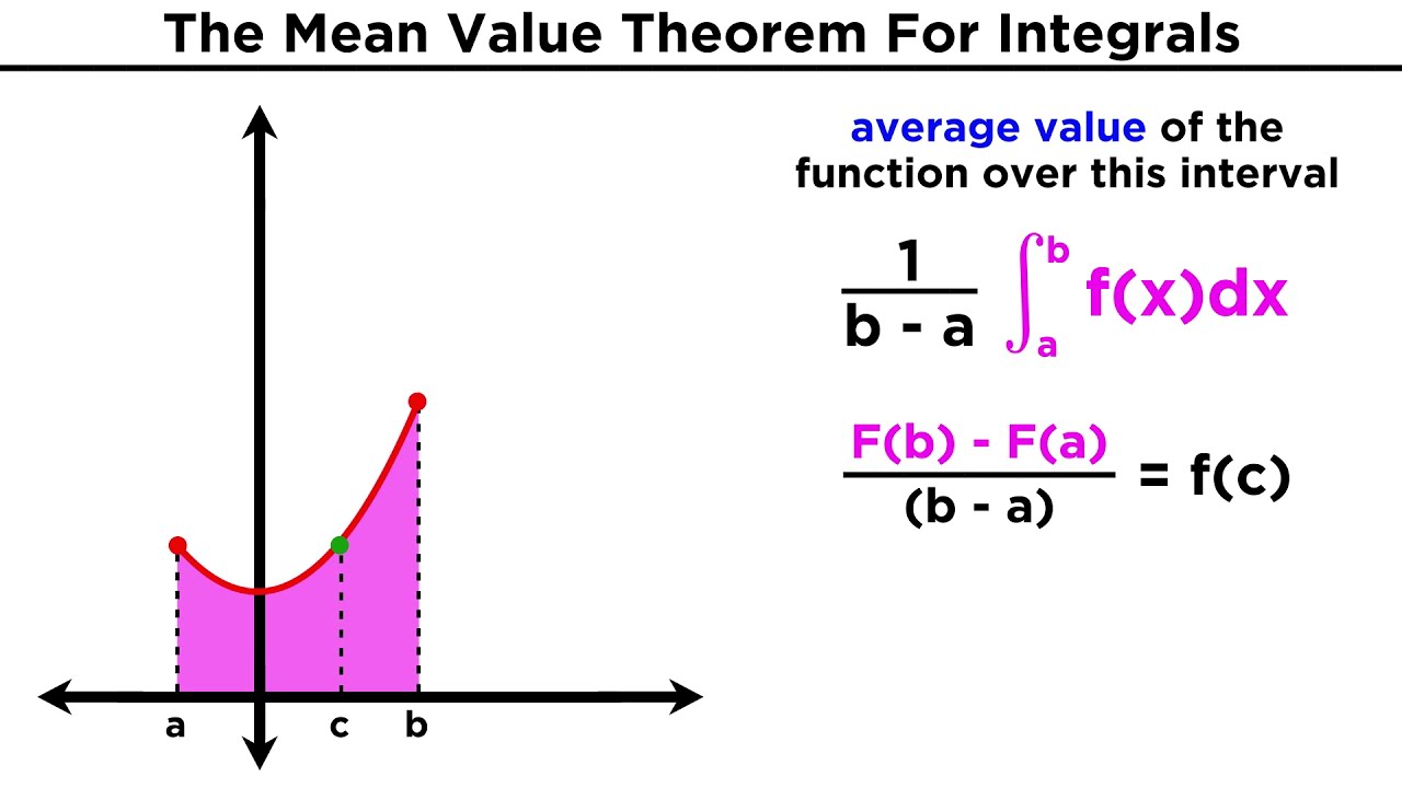
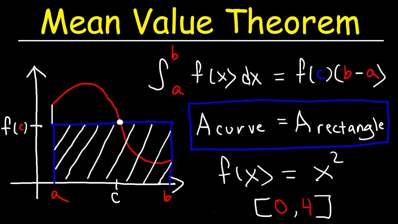
- 🔍 The value 'c' in the average value formula (1/(b-a) * ∫[a to b] f(x) dx) represents the x-value where the area under the curve equals the area of the rectangle.
- 📌 In the case of the function f(x) = 2x + 1 from x=1 to x=5, the average value is 7, which is the same as the average y-value.
- 🚫 For non-linear functions, the average value of the function may not equal the average y-value.
- 📶 The average value of the function can be greater, less than, or equal to the average y-value depending on the shape of the curve.
- 🌡️ For the function f(x) = x^2 from x=0 to x=4, the average value is approximately 5.33, which is less than the average y-value of 8.
- 🌱 For the function f(x) = √x from x=4 to x=16, the average value is 28/9, which is greater than the average y-value of 3.
- 📍 The value of 'c' does not always correspond to the midpoint of the interval 'a' and 'b', especially for non-linear functions.
- 🔧 The process of finding 'c' involves taking the square root of the average value and solving for 'x' when f(x) is not a linear function.
- 🔍 Analyzing the secant line in relation to the curve of the function can help understand why the average function value may vary from the average y-value.
Q & A
What is the given linear function in the script?
-The given linear function is f(x) = 2x + 1.
What is the interval considered for finding the average value of the function?
-The interval considered is from 1 to 5.
How is the average value of a function over an interval defined?
-The average value of a function over an interval is defined as (1 / (b - a)) * ∫[a to b] f(x) dx, where 'a' and 'b' are the endpoints of the interval.
What is the y-intercept of the given linear function?
-The y-intercept of the given linear function is 1.
What is the slope of the linear function?
-The slope of the linear function is 2.
What is the average y value for the linear function over the interval [1, 5]?
-The average y value for the linear function over the interval [1, 5] is 7.
How does the average value of a linear function compare to the average y value?
-For a linear function, the average value of the function is equal to the average y value over the interval from 'a' to 'b'.
What is the average x value for the interval [1, 5]?
-The average x value for the interval [1, 5] is 3, which is the midpoint of the interval.
What is the value of 'c' for the linear function that makes the area under the curve equal to the area of the rectangle?
-For the linear function, 'c' is equal to the average x value, which is 3.
How does the average value of a function change if the function is not linear?
-If the function is not linear, the average value of the function may not be equal to the average y value. It depends on the shape of the curve relative to the secant line between the interval endpoints.
What is the significance of the value 'c' in the context of the mean value theorem?
-In the context of the mean value theorem, 'c' is the value at which the function's value equals the average value over the interval, making the area under the curve equal to the area of the rectangle formed by the secant line and the x-axis.
Outlines
📊 Calculating the Average Value of a Linear Function
This paragraph discusses the method of finding the average value of a linear function, f(x) = 2x + 1, over the interval from 1 to 5 using a straw graph and the mean value theorem. It explains that the average value corresponds to the y-coordinate of the point where the area under the curve equals the area of the rectangle with height f(c) and width (b-a). The calculation involves evaluating the definite integral from a to b and dividing by (b-a), resulting in an average value of 7, which is the same as the average y-value in the interval for a linear function.
📈 Comparing Average Values for Non-Linear Functions
The second paragraph explores the concept of average value for non-linear functions, using the example of f(x) = x^2 over the interval from 0 to 4. It contrasts the average y-value (8) with the average function value (approximately 5.33), highlighting that for non-linear functions, the average function value may not equal the average y-value. The paragraph also introduces the concept of the average x-value and demonstrates how to calculate the value of c that corresponds to the average function value, which is found to be approximately 2.309, greater than the average x-value of 2.
🌟 Analyzing Function Behavior with Average Values
This paragraph delves into the behavior of functions by comparing their average values with the average y-values over specified intervals. It presents a third example with f(x) as the square root of x over the interval from 4 to 16 and shows that the average function value (approximately 3.1) can be greater than the average y-value (3). The paragraph emphasizes that for linear functions, the average function value equals the average y-value, but this relationship varies for non-linear functions. It visually represents the three functions graphed and explains how the position of the curve relative to the secant line affects the relationship between the average function value and the average y-value.
Mindmap
Keywords
💡Linear Function
💡Mean Value Theorem
💡Definite Integral
💡Average Value
💡Y-Intercept
💡Slope
💡Interval
💡Anti-Derivative
💡Area Under the Curve
💡Secant Line
💡Midpoint
Highlights
Exploring the average value of a linear function f(x) = 2x + 1 over the interval [1, 5].
Using the Mean Value Theorem to find the average value of a function.
Calculating the area under the curve as the definite integral from a to b.
Deriving the formula for the average value as 1/(b-a) * integral from a to b of f(x) dx.
For a linear function, the average value is the average y-value in the interval a to b.
Finding c for the linear function, where the area under the curve equals the area of the rectangle.
The average value of the function is 7, which is the average y-value for the interval [1, 5].
Analyzing a non-linear function, f(x) = x^2, over the interval [0, 4].
Comparing the average value of the function to the average y-value and finding that they are different for non-linear functions.
Calculating the average value for f(x) = x^2 as 16/3, which is less than the average y-value of 8.
For the function f(x) = sqrt(x), finding the average value over the interval [4, 16] to be 28/9, greater than the average y-value of 3.
Observing that c for non-linear functions is not the midpoint of a and b, and the average function value is not the average y-value.
Drawing graphs for the three functions to visualize the relationship between average function value and average y-value.
Understanding that for a linear function, the average function value equals the average y-value, but this does not hold for non-linear functions.
Noting that the position of c relative to the average x-value depends on the nature of the function.
The average function value can be less than, equal to, or greater than the average y-value depending on the function's shape.
The significance of the function's shape in determining the relationship between the average function value and the average y-value.
Practical applications of understanding average values in various types of functions for problem-solving and analysis.
Transcripts
Browse More Related Video
The Mean Value Theorem For Integrals: Average Value of a Function
Mean Value Theorem For Integrals

Calculus: Average Value of a Function (Section 6.5) | Math with Professor V

Average Value of a Continuous Function

Average Value of a Continuous Function on an Interval

Mean value theorem for integrals | AP Calculus AB | Khan Academy
5.0 / 5 (0 votes)
Thanks for rating: