Mean Value Theorem For Integrals
TLDRThe video script discusses the Mean Value Theorem for Integrals, illustrating how a function's definite integral over an interval can be represented by the area under a rectangle with a height equal to the function's value at some point 'c'. Through examples, the script demonstrates how to find 'c' for different functions, such as x squared, square root of x, and linear functions, showing that 'c' aligns with the midpoint for linear functions and may vary for others based on concavity. The detailed mathematical steps and explanations engage viewers in understanding this fundamental theorem's practical applications.
Takeaways
- 📌 The Mean Value Theorem for Integrals states that for a continuous function on a closed interval [a, b], there exists a point 'c' where the area under the curve is equal to the area of a rectangle.
- 📈 The definite integral of a function from 'a' to 'b' is represented as ∫(f(x)dx) from 'a' to 'b', and it corresponds to the area under the curve.
- 🌟 If a function is continuous on [a, b], the Mean Value Theorem guarantees that there is at least one value 'c' in the interval where the average value equals the function's value at 'c'.
- 🔢 For the function f(x) = x^2 over the interval [0, 4], the value of 'c' is found to be +/- (4 * √3) / 3, ensuring it lies within the interval [0, 4].
- 📊 For the function f(x) = √x over the interval [1, 9], the value of 'c' is calculated to be approximately 4.694, which is less than the midpoint 5 but within the interval [1, 9].
- 🌐 For a linear function f(x) = 2x + 3 over the interval [2, 10], the value of 'c' is equal to the midpoint of the interval, which is 6.
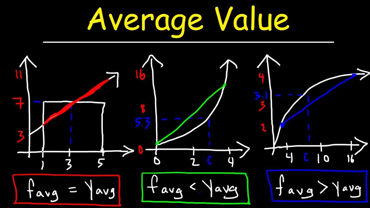
- 📂 The position of 'c' relative to the midpoint varies depending on the concavity of the function: for a function that is increasing and concave up, 'c' is greater than the midpoint; for one that is increasing and concave down, 'c' is less than the midpoint.
- 🧩 The Mean Value Theorem is a fundamental concept in calculus that links the behavior of a function to its integral over a certain interval.
- 🔍 The theorem can be applied to find specific points on a curve that have particular geometric or analytical properties, such as representing the average value of a function over an interval.
- 📝 The process of finding 'c' involves setting up and solving equations that equate the area under the curve to the area of a rectangle, using the properties of integrals and antiderivatives.
- 📊 Understanding the Mean Value Theorem and its implications is crucial for analyzing a wide range of mathematical and real-world problems, from physics to engineering and economics.
Q & A
What is the Mean Value Theorem for Integrals?
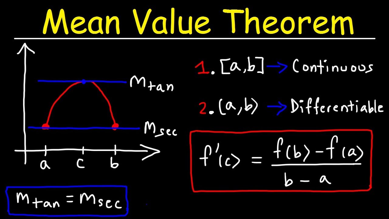
-The Mean Value Theorem for Integrals states that if a function is continuous on a closed interval [a, b], then there exists at least one point 'c' in that interval such that the area under the curve from 'a' to 'b' is equal to the rectangle formed with the width (b-a) and the height (f(c)). Mathematically, this means that the definite integral of f(x) dx from 'a' to 'b' is equal to f(c) * (b-a).
How does the Mean Value Theorem for Integrals relate to rectangles and curves?
-The Mean Value Theorem for Integrals relates rectangles and curves by stating that for a continuous function on a closed interval, there is a point 'c' where the area under the curve (which is the definite integral) is equal to the area of a rectangle with base (b-a) and height f(c). This illustrates that the definite integral can be thought of as the 'area' of the curve over the interval [a, b].
What is the antiderivative of x^2?
-The antiderivative of x^2 is (1/3)x^3. This is found using the power rule for integration, which states that the integral of x^n dx is (1/(n+1))x^(n+1), where n is a constant.
How do you find the value of 'c' for a function f(x) = x^2 on the interval [0, 4]?
-To find the value of 'c' for f(x) = x^2 on [0, 4], you first evaluate the integral of x^2 from 0 to 4 and set it equal to f(c) * (4-0). By calculating the antiderivative and applying the bounds, you get (4^3)/3 - (0^3)/3 = 64/3. Solving for c, you find that c = ±(4 * sqrt(3))/3. Since c must be within the interval [0, 4], the valid value for 'c' is (4 * sqrt(3))/3.
What is the antiderivative of the square root of x?
-The antiderivative of the square root of x, or √x, is (2/3)x^(3/2). This is found using the power rule for integration with a fractional exponent, which involves multiplying the coefficient by the exponent and raising the base to the new exponent.
How do you calculate the value of 'c' for a function f(x) = √x on the interval [1, 9]?
-To calculate the value of 'c' for f(x) = √x on [1, 9], you set up the equation based on the Mean Value Theorem for Integrals, solve the integral of √x from 1 to 9, and equate it to f(c) * (9-1). After evaluating the integral and solving for 'c', you find that 'c' equals the square root of the ratio of the integral's value to (9-1), which results in √(52/8) or approximately 4.694.
What is the general formula for the antiderivative of a linear function like f(x) = 2x + 3?
-The antiderivative of a linear function f(x) = 2x + 3 is F(x) = x^2 + 3x. This is derived using the power rule for integration, which applies to each term in the function separately.
What is the expected value of 'c' for a linear function on the interval [a, b]?
-For a linear function, the expected value of 'c' where the area of the rectangle is equal to the area under the curve is the midpoint of the interval [a, b]. This is because a linear function does not curve upwards or downwards, so the average rate of change is consistent throughout the interval.
How does the position of 'c' relate to the concavity of a function?
-The position of 'c' relative to the midpoint of the interval [a, b] depends on the concavity of the function. If the function is concave up, 'c' will be to the right of the midpoint. If the function is concave down, 'c' will be to the left of the midpoint. For functions that are neither concave up nor down (like linear functions), 'c' will be equal to the midpoint.
What are the intervals and corresponding 'c' values for the three examples provided in the script?
-For the function f(x) = x^2 on the interval [0, 4], 'c' is approximately (4 * sqrt(3))/3. For f(x) = √x on [1, 9], 'c' is about 4.694. Lastly, for the linear function f(x) = 2x + 3 on [2, 10], 'c' is exactly at the midpoint, which is 6.
What is the significance of the Mean Value Theorem for Integrals in calculus?
-The Mean Value Theorem for Integrals is significant in calculus as it provides a fundamental relationship between the area under a curve and the average value of a function over an interval. It helps in understanding the concept of definite integrals and their geometric interpretation, as well as offering a powerful tool for solving problems in calculus and analysis.
How does the Mean Value Theorem for Integrals apply to non-linear functions?
-For non-linear functions, the Mean Value Theorem for Integrals ensures that there exists a 'c' in the interval [a, b] where the average value of the function over that interval is equal to the function's value at 'c'. This theorem is particularly useful for functions that are not linear, as their rate of change varies throughout the interval, and it helps in approximating the area under the curve.
Outlines
📚 Introduction to the Mean Value Theorem for Integrals
This paragraph introduces the Mean Value Theorem for Integrals, explaining its basic concept through a visual representation. It describes a scenario where a function is represented on a graph from point 'a' to 'b', and a rectangle is drawn under the curve with its width 'b-a' and height 'f(c)'. The theorem states that for a continuous function on a closed interval 'a' to 'b', there exists a point 'c' where the area of the rectangle equals the area under the curve. The definite integral of 'f(x)dx from a to b' is given by 'f(c) * (b-a)', signifying that 'f(c)' represents the average value of the function over the interval. The paragraph then applies this concept to a specific function, f(x) = x^2, over the interval [0,4], to find the value of 'c' guaranteed by the theorem. The process involves calculating the antiderivative of f(x), setting it equal to the area under the curve, and solving for 'c'. The result is 'c' = ±(4 * √3)/3, but since 'c' must be within the interval [0,4], the valid answer is 'c' = (4 * √3)/3.
🧠 Solving for 'c' in Different Functions
This paragraph continues the exploration of the Mean Value Theorem for Integrals by applying it to two additional functions. The first function is f(x) = √x over the interval [1,9]. The process involves rewriting the function for integration, calculating the antiderivative, and solving for 'c'. The result is 'c' = √(13/6), which falls within the interval [1,9]. The second function is a linear function, f(x) = 2x + 3, over the interval [2,10]. The paragraph discusses a general rule that for linear functions, 'c' will be equal to the midpoint of the interval 'a' to 'b'. The calculation confirms this rule, showing that 'c' = 6, which is the midpoint of [2,10]. The paragraph concludes by comparing the three problems, highlighting how the position of 'c' relative to the midpoint varies depending on the concavity of the function.
📈 Comparing 'c' Values in Different Scenarios
The final paragraph of the script summarizes and compares the 'c' values found in the three different functions discussed earlier. It emphasizes the relationship between the shape of the function (concave up, concave down, or linear) and the position of 'c' relative to the midpoint of the interval 'a' to 'b'. For the quadratic function f(x) = x^2, 'c' was to the right of the midpoint, showing an increase in the function that is concave up. For the square root function f(x) = √x, 'c' was to the left of the midpoint, indicating an increasing function that is concave down. For the linear function f(x) = 2x + 3, 'c' was equal to the midpoint, which is expected for a function that is neither concave up nor down. This comparison provides a clear understanding of how the Mean Value Theorem manifests in different types of functions, reinforcing the concept's versatility and importance in calculus.
Mindmap
Keywords
💡Mean Value Theorem for Integrals
💡Definite Integral
💡Antiderivative
💡Continuous Function
💡Rectangle Area
💡Power Rule
💡Midpoint
💡Concavity
💡Linear Function
💡Interval
💡Rationalize
Highlights
Mean Value Theorem for Integrals is discussed in the video.
A function is presented with a specific area under the curve being equal to the area of a rectangle.
The Mean Value Theorem states that for a continuous function on a closed interval, there exists a point c where the area under the curve equals the area of the rectangle.
The definite integral is represented as the area under the curve.
The first example involves a function f(x) = x^2 over the interval [0, 4] and finding the value of c.
The antiderivative of x^2 is found using the power rule, resulting in x^3/3.
The value of c for the x^2 function is calculated to be ±(4 * sqrt(3))/3, but only the positive value is within the interval [0, 4].
The second example features the function f(x) = sqrt(x) on the interval [1, 9].
The value of c for the square root function is determined to be approximately 4.694, which is within the interval [1, 9].
For the third example, a linear function f(x) = 2x + 3 over the interval [2, 10] is analyzed.
It is hypothesized that for a linear function, the value of c is equal to the midpoint of the interval [a, b].
The value of c for the linear function is confirmed to be 6, which is the midpoint of [2, 10].
The Mean Value Theorem for Integrals guarantees a value of c where the rectangle's area equals the curve's area for any continuous function.
For functions that are concave up, c is greater than the midpoint; for those concave down, c is less than the midpoint.
The video provides a comprehensive explanation of the Mean Value Theorem for Integrals with clear examples.
The mathematical concepts are broken down into manageable steps, making the theorem accessible to viewers.
The video demonstrates the application of the Mean Value Theorem to different types of functions, highlighting its versatility.
The use of visual aids, such as graphs and rectangles, helps in understanding the theorem's implications.
The video's approach to explaining the theorem is both educational and engaging, suitable for a range of audiences.
The video concludes by comparing the three examples, reinforcing the key concepts and differences between the functions.
Transcripts
Browse More Related Video
5.0 / 5 (0 votes)
Thanks for rating: