Simple Linear Regression Concept | Statistics Tutorial #32 | MarinStatsLectures
TLDRThis video introduces the basics of simple linear regression, a statistical method to model the relationship between two variables. It explains how to use gestational age and head circumference of babies as an example to illustrate the concept. The video emphasizes the difference between correlation and regression, highlighting that while correlation indicates the direction and strength of a relationship, regression allows for prediction and estimation of outcomes. It also discusses the importance of understanding the slope and intercept in a regression model and touches on the goals of regression analysis, whether it's to estimate the effect of a variable or to predict outcomes. The video concludes by noting that linear regression is a vast topic with many applications and assumptions that will be explored in more depth later.
Takeaways
- 📊 Simple linear regression is an introductory statistical method used to model the relationship between two variables, where one is numeric and continuous, such as gestational age and head circumference.
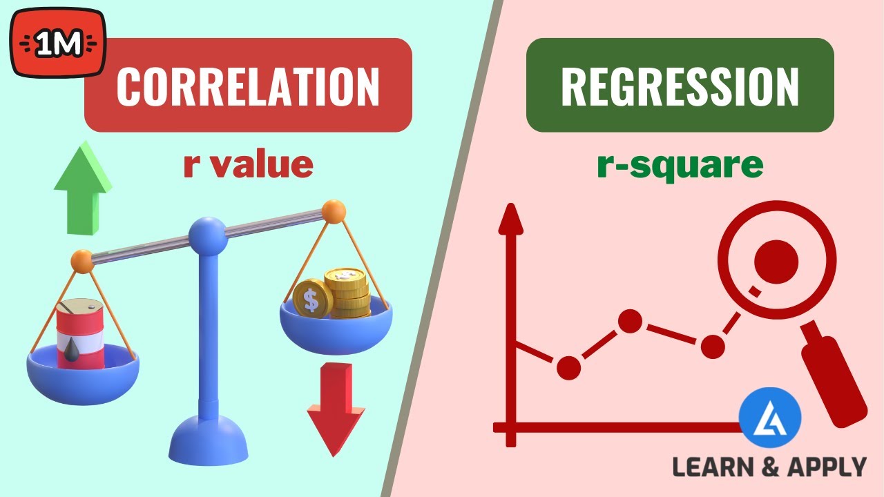
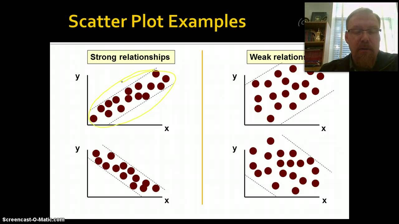
- 🔗 The correlation coefficient indicates the direction and strength of the linear association between variables but does not imply causation or the effect of one variable on the other.
- 📈 Linear regression models Y as a linear function of X, aiming to fit a line (the regression line) through the data points to estimate or predict Y values based on X.
- 🎯 The key components of a simple linear regression model include the slope (b1), the y-intercept (b0), and the residuals (errors), which represent the difference between observed and predicted Y values.
- 📐 The slope (b1) in a regression line is calculated as the correlation coefficient multiplied by the ratio of the standard deviation of Y to the standard deviation of X, indicating the change in Y for a one-unit change in X.
- 🏁 The y-intercept (b0) represents the estimated Y value when X is zero, which may not always have a meaningful interpretation, especially when X has not been observed at zero.
- 🔄 The method of least squares is commonly used to define the best-fit line by minimizing the sum of squared residuals, which is equivalent to maximizing the likelihood of the observed data.
- 🎯 Two primary goals of regression models are either to estimate the effect of X on Y (effect size model) or to predict the outcome Y given an X value (predictive model).
- 🔄 Assumptions underpinning linear regression models will be explored separately, including how to check and address potential violations, and alternative approaches when assumptions are not met.
- 🌐 Linear regression is a vast topic that can encompass entire courses, and this introduction serves as a foundation for further exploration and understanding of more complex regression models.
Q & A
What is the primary purpose of simple linear regression?
-The primary purpose of simple linear regression is to model the relationship between two variables, typically when one variable (Y) is numeric or continuous and the other (X) is also numeric or continuous. It helps in understanding how changes in the independent variable (X) are associated with changes in the dependent variable (Y).
What is the difference between the X and Y variables in simple linear regression?
-In simple linear regression, the X variable is the independent variable, which is believed to influence the Y variable. The Y variable is the dependent variable, which is the outcome that is being predicted or explained by the independent variable. While both variables are usually numeric or continuous, the X variable can also be categorical or a factor.
How is Pearson's correlation related to simple linear regression?
-Pearson's correlation coefficient measures the strength and direction of the linear relationship between two variables. In simple linear regression, it is used to summarize the association between the X and Y variables. However, while it indicates the strength of the linear association, it does not allow us to make predictions or estimate the effect of X on Y.
What does the slope (b1) in a simple linear regression model represent?
-The slope (b1) in a simple linear regression model represents the amount of change in the dependent variable (Y) for a one-unit change in the independent variable (X). It is calculated as the correlation between X and Y multiplied by the ratio of the standard deviation of Y to the standard deviation of X.
What is the y-intercept (b0) in a simple linear regression model, and what does it represent?
-The y-intercept (b0) in a simple linear regression model represents the estimated value of Y when X is zero. It is calculated as the mean of Y minus the slope (b1) times the mean of X. However, the y-intercept may not always have a meaningful interpretation, especially when X has not been observed at zero.
What are the two broad goals for building a simple linear regression model?
-The two broad goals for building a simple linear regression model are estimation and prediction. Estimation involves understanding the effect of the independent variable (X) on the dependent variable (Y), while prediction focuses on using the model to forecast the value of Y based on given values of X.
How is the method of least squares used in simple linear regression?
-The method of least squares is used to define the best-fit line in simple linear regression by minimizing the sum of squared errors (residuals) between the observed Y values and the predicted Y values. This method results in a line that best represents the relationship between X and Y while minimizing the overall deviation of the data points from the line.
What is the difference between an error and a residual in the context of simple linear regression?
-In the context of simple linear regression, an error generally refers to the theoretical difference between the actual Y value and the true predicted Y value, while a residual is the observed difference between the actual Y value and the predicted Y value from the regression line. Although the terms are sometimes used interchangeably, the distinction lies in whether one is referring to theoretical errors or observed residuals.
How can the assumptions for a simple linear regression model be checked and addressed if not met?
-The assumptions for a simple linear regression model include linearity, independence of errors, constant variance of errors (homoscedasticity), and normality of errors. These assumptions can be checked using diagnostic plots, statistical tests, and residual analysis. If the assumptions are not met, alternative models or transformation techniques may be employed to address the violations and improve the model's fit and validity.
What is the role of the standard deviation in calculating the slope (b1) in a simple linear regression model?
-The standard deviation plays a crucial role in scaling the correlation to account for the units of measurement. The slope (b1) is calculated as the correlation multiplied by the ratio of the standard deviation of Y to the standard deviation of X. This scaling ensures that the slope represents the change in Y per unit change in X, taking into account the variability and units of both variables.
How can the interpretation of the y-intercept (b0) be made more meaningful?
-The interpretation of the y-intercept (b0) can be made more meaningful by centering the X variable. Centering involves selecting a reference point within the observed range of X and considering it as the 'zero' value. This technique allows for a more intuitive understanding of where the regression line crosses the Y-axis and can provide a meaningful estimate of Y when X is at the reference point.
Outlines
📊 Introduction to Simple Linear Regression
This paragraph introduces the concept of simple linear regression, explaining its use when both X and Y variables are numeric or continuous. It sets the stage for understanding regression models by using the example of gestational age and head circumference in low birth weight babies. The paragraph also discusses the limitations of Pearson's correlation coefficient and emphasizes the importance of building a model to estimate Y as a linear function of X, highlighting the foundational role of simple linear regression in understanding more complex models.
📈 Understanding Regression Terminology and Concepts
This section delves into the terminology and concepts of simple linear regression, including observed values (xi, yi), estimated values (yi^), and residuals (ei). It explains the regression line as the estimated mean of Y given X (b0 + b1X) and discusses the difference between modeling individuals and estimating the mean for a population. The paragraph also touches on the interchangeable use of the terms error and residual, and the importance of understanding the difference between theoretical errors and observed errors in a dataset.
🧠 Slope and Intercept Interpretation in Regression
This paragraph focuses on the interpretation of the slope (b1) and intercept (b0) in a regression line. It explains how the slope is calculated as the correlation times the standard deviation of Y over the standard deviation of X, and how this represents the change in Y for a one-unit change in X. The intercept is described as the estimated Y value when X equals zero, with a discussion on its potential lack of meaningful interpretation, especially when X has not been observed at zero. The paragraph also briefly mentions the method of least squares and maximum likelihood as approaches to defining the best line.
🎯 Goals and Assumptions of Regression Modeling
The final paragraph discusses the two broad goals of regression modeling: estimating the effect of X on Y (effect size model) and predicting the outcome (predictive model). It provides an example of how to use the regression equation to predict head circumference based on gestational age. The paragraph also mentions the necessary assumptions for building a linear regression model, the importance of checking these assumptions, and the potential need for alternative approaches if assumptions are not met. It concludes by acknowledging the complexity of linear regression as a topic and the intention to build on the concepts introduced throughout the course.
Mindmap
Keywords
💡Simple Linear Regression
💡Numeric or Continuous Variables
💡Pearson's Correlation
💡Correlation Coefficient
💡Regression Line
💡Residual
💡Y-Intercept
💡Slope
💡Modeling
💡Effect Size
💡Predictive Model
Highlights
Simple linear regression is introduced as a foundational concept for understanding regression models.
The X variable in simple linear regression can be either numeric/continuous or categorical/factor.
The video uses the example of gestational age (X) and head circumference (Y) of low birth weight babies to illustrate the concepts.
Pearson's correlation is discussed as a measure of the direction and strength of association but not the effect of X on Y.
The concept of modeling Y as a linear function of X is central to linear regression.
George Box's famous quote about models being wrong but some useful is mentioned, emphasizing the simplifications in models.
Simple linear regression serves as a stepping stone to more complex models like generalized linear models and logistic regression.
The terminology of observed X and Y values, estimated Y values (Y-hat), and residuals (errors) is introduced.
The equation of the regression line is defined with a y-intercept (b-not) and a slope (b1).
The method of least squares is mentioned as a technique to define the best-fit line by minimizing the sum of squared errors.
The slope (b1) of the regression line is explained as the correlation times the standard deviation of Y over the standard deviation of X.
The y-intercept (b-not) is described as the estimated Y value for X equals zero, which may not always have a meaningful interpretation.
The goals of a regression model are outlined, including estimating the effect of X on Y and predictive modeling.
The importance of assumptions in building a linear regression model is acknowledged, with a promise to explore them further in the course.
Linear regression is recognized as a vast topic that can encompass multiple courses in itself.
Transcripts
Browse More Related Video
Correlation and Regression Analysis: Learn Everything With Examples
10.2.1 Regression - Essential Terminology and Background Related to Regression
Simple Linear Regression in R | R Tutorial 5.1 | MarinStatsLectures

Elementary Stats Lesson #5

Video 1: Introduction to Simple Linear Regression
Introduction to Correlation & Regression, Part 1
5.0 / 5 (0 votes)
Thanks for rating: