Velocity Time Graphs, Acceleration & Position Time Graphs - Physics
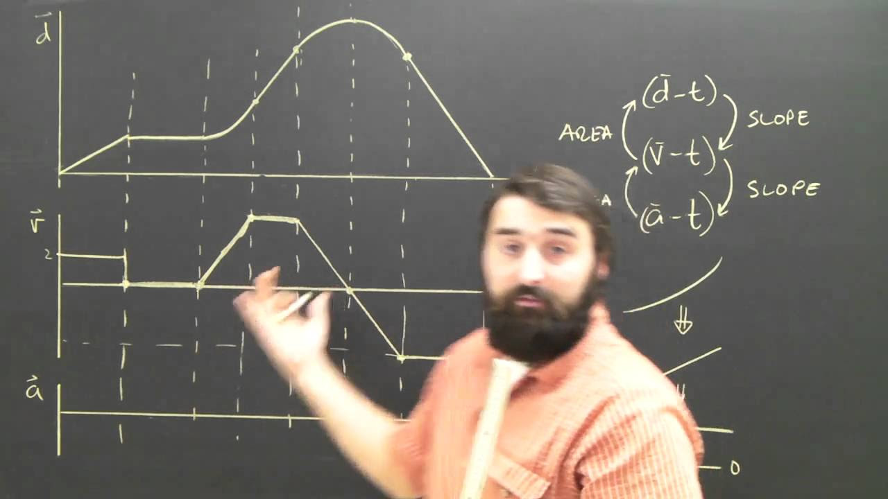
TLDRThis video script delves into the concepts of motion graphs, focusing on position-time, velocity-time, and acceleration-time graphs. It explains the significance of slope and area in these graphs, associating slope with division (representing velocity and acceleration) and area with multiplication (representing displacement and change in velocity). The script clarifies that the slope of a position-time graph indicates instantaneous velocity, the area under a velocity-time graph represents displacement, and the area under an acceleration-time graph signifies the change in velocity. It also distinguishes between position-time and distance-time graphs, emphasizing the importance of understanding these concepts for solving physics problems involving motion.
Takeaways
- 📈 The slope in a position-time graph represents velocity, calculated as the change in position (y) divided by the change in time (x).
- 📊 The area under a position-time graph does not provide useful information in physics, as it represents a multiplication of meters and seconds, which does not relate to displacement.
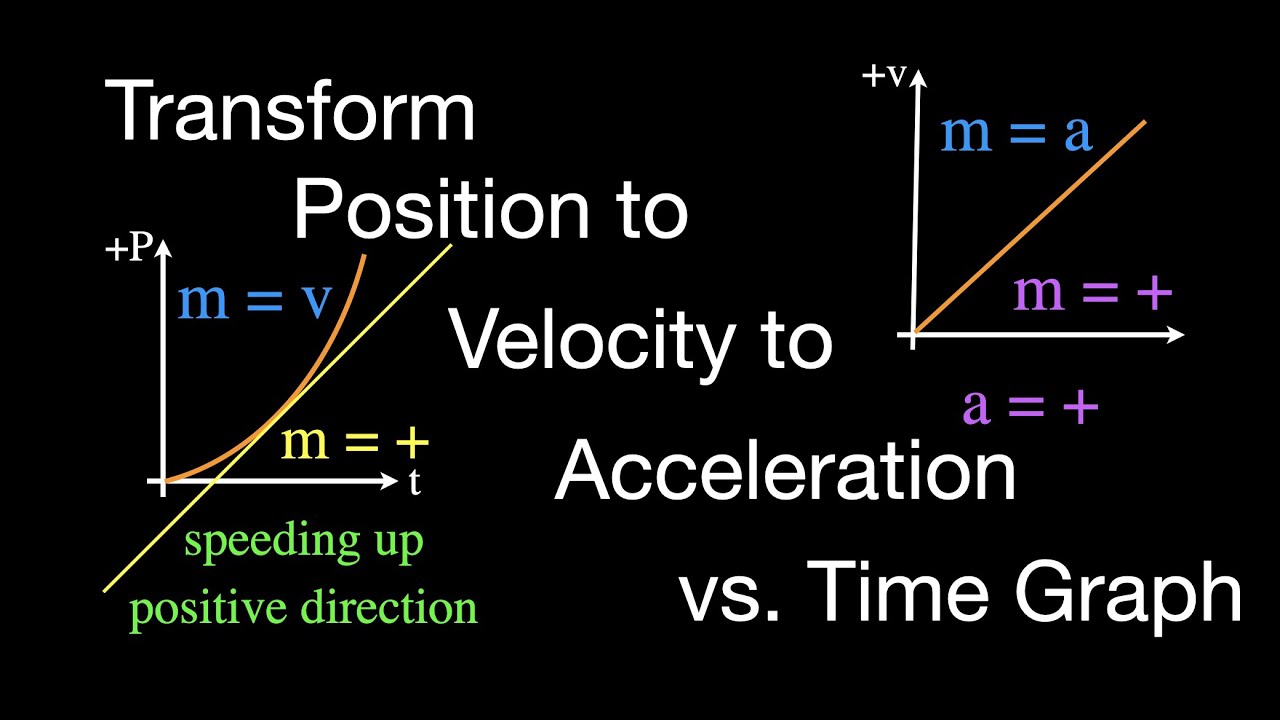
- 🚀 The slope of a velocity-time graph is acceleration, derived from the change in velocity divided by the change in time.
- 📐 The area under a velocity-time graph equals displacement, calculated by multiplying velocity by time.
- 🔄 The slope of an acceleration-time graph is jerk (rate of change of acceleration), which is not commonly used in everyday physics.
- 🔄 The area under an acceleration-time graph represents the change in velocity, found by multiplying acceleration by time.
- 📈📊 The difference between position-time and distance-time graphs is that the slope of the former represents velocity, while the slope of the latter represents speed.
- 🔄 For linear (straight) position-time graphs, the slope is constant, indicating constant velocity and zero acceleration.
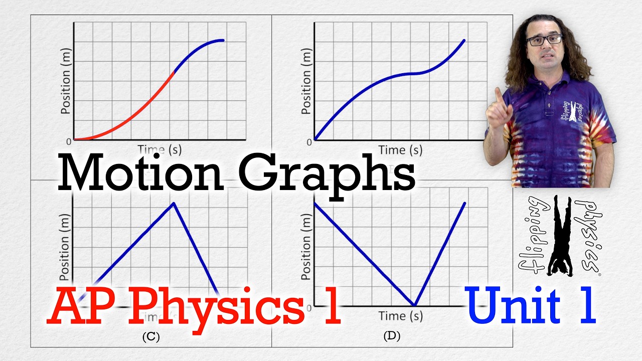
- 📈📊 In parabolic position-time graphs, the concavity indicates the sign of acceleration (negative for concave down, positive for concave up).
- 🚦 The direction of velocity (positive or negative) and its change (increasing or decreasing) can be determined from the shape of the position-time graph.
- 🚦 An object is speeding up when acceleration and velocity have the same sign, and slowing down when they have opposite signs.
Q & A
What are the two fundamental concepts related to graphs that the video discusses?
-The two fundamental concepts discussed in the video are slope and area. The slope is associated with division, while the area is associated with multiplication.
How is the slope of a position-time graph related to velocity?
-The slope of a position-time graph represents the velocity of the object at any given moment. If you calculate the slope at a specific point, it gives you the instantaneous velocity, and if you calculate it using two points, it gives you the average velocity.
What does the area under a velocity-time graph represent?
-The area under a velocity-time graph represents the displacement of the object. Displacement is the final position minus the initial position.
How can you differentiate between instantaneous and average velocity?
-Instantaneous velocity is found by calculating the slope of the tangent line to the position-time graph at a specific point, while average velocity is found by calculating the slope of the secant line connecting two points on the graph.
What does the slope of an acceleration-time graph represent?
-The slope of an acceleration-time graph represents the rate of change of acceleration, which is also known as 'jerk' or 'jolt' in physics.
What does the area under an acceleration-time graph represent?
-The area under an acceleration-time graph represents the change in velocity, which is the final velocity minus the initial velocity.
How can you determine if an object is speeding up or slowing down based on acceleration and velocity?
-An object is speeding up when the acceleration and velocity have the same sign (both positive or both negative), and it is slowing down when they have opposite signs.
What are the three linear shapes of a position-time graph and what do they indicate about velocity and acceleration?
-The three linear shapes are a straight line going up, a horizontal line, and a straight line going down. These shapes indicate constant velocity (positive, zero, or negative respectively) and zero acceleration since the slope is constant.
What are the four parabolic shapes of a position-time graph and what do they indicate about velocity and acceleration?
-The four parabolic shapes are concave up, concave down, a combination of both forming a 'U' shape, and the reverse. These shapes indicate changing velocity and non-zero acceleration, with the direction of the curve indicating the sign of acceleration (positive for concave up and negative for concave down).
How does the shape of a position-time graph indicate whether an object is at rest or changing direction?
-A horizontal position-time graph indicates that the object is at rest or changing direction. If the graph is momentarily horizontal before changing direction (up or down), it indicates that the object is at rest for a brief moment or transitioning between directions.
What is the relationship between speed and velocity?
-Speed is the absolute value of velocity and is always positive. Velocity, on the other hand, can be positive or negative, indicating the direction of motion along the x-axis. Speed measures how fast an object is moving, while velocity includes the direction of motion.
Outlines
📈 Introduction to Motion Graphs and Concepts of Slope and Area
This paragraph introduces the topic of motion graphs, specifically focusing on position-time, velocity-time, and acceleration-time graphs. It emphasizes the importance of understanding the concepts of slope and area, where slope is related to division (change in y/x) and area to multiplication (length * width). The paragraph explains how the slope of a position-time graph represents velocity, either instantaneous or average, depending on whether it's the slope of the tangent or secant line. The area under a position-time graph, however, is not useful in physics as it results in a unit of meters times seconds, which doesn't provide meaningful information. The paragraph sets the foundation for further discussion on how these concepts apply to different types of motion graphs.
🏃♂️ Velocity-Time Graphs and Their Interpretation
The second paragraph delves into the velocity-time (VT) graph, explaining that the slope of a VT graph represents acceleration, calculated by the change in velocity over the change in time. The area under a VT graph is significant, as it represents displacement, the final position minus the initial position. The paragraph clarifies that multiplying velocity (y-axis) by time (x-axis) yields displacement in meters. It also introduces the concept that the area under a VT graph can be used to determine the displacement when the velocity is multiplied by time, which is a crucial concept in understanding motion along the x-axis.
🚀 Acceleration-Time Graphs and Jerk
This paragraph discusses acceleration-time (AT) graphs, highlighting that the slope of an AT graph represents the rate of change of acceleration, a concept known as jerk. While jerk is not commonly encountered in most physics courses, it's essential to understand that the slope of an AT graph can represent this concept. The area under an AT graph is also explored, explaining that it represents the change in velocity, calculated by the final velocity minus the initial velocity. The paragraph emphasizes the importance of distinguishing between a position-time graph and an acceleration-time graph, as the former gives velocity and the latter gives the change in velocity.
📊 Understanding Tangent and Secant Lines for Velocity Calculation
The fourth paragraph focuses on the mathematical and conceptual approach to finding the instantaneous and average velocity using tangent and secant lines on a position-time graph. It explains that the slope of the tangent line at a specific point gives the instantaneous velocity, while the slope of the secant line between two points provides the average velocity. The paragraph also discusses the practicality of approximating the slope of the tangent line using the secant line's slope, especially when the two points used for the secant line are very close to the point of interest. This approximation allows for a more accurate calculation of instantaneous velocity.
🔄 Direction and Magnitude of Velocity and Acceleration
The fifth paragraph explores the implications of the direction and magnitude of velocity and acceleration on a position-time graph. It explains how the direction of position change (increasing or decreasing) determines the sign of velocity (positive or negative), which in turn indicates the direction of motion along the x-axis. The paragraph also discusses how the velocity's sign can indicate rest or change in direction when it is zero. Furthermore, it describes how the relationship between the signs of acceleration and velocity indicates whether an object is speeding up or slowing down, with the same signs indicating acceleration and opposite signs indicating deceleration.
📈 Analyzing Position-Time Graph Shapes and Their Kinematic Implications
The sixth paragraph examines different shapes of position-time graphs and their corresponding kinematic meanings. It categorizes the graphs into linear and parabolic shapes, explaining that linear shapes indicate constant velocity and hence zero acceleration. The paragraph then associates specific shapes with the direction of motion and the signs of velocity and acceleration. For parabolic shapes, the paragraph describes how the concavity of the graph can be used to determine the sign of acceleration. It also connects the change in slope of the graph to the rate of change of velocity, providing a method to analyze whether the motion is speeding up or slowing down based on the concavity and the direction of the slope change.
🚦 Summarizing Position-Time Graph Analysis
The final paragraph summarizes the key points from the previous discussion on position-time graphs. It reiterates the methods to determine the sign of velocity, the calculation of acceleration, and the determination of whether an object is speeding up or slowing down. The paragraph emphasizes the ability to answer almost any question related to position-time graphs by understanding the signs of velocity and acceleration, the increasing or decreasing nature of velocity, and the interpretation of the graph's linear or parabolic shapes. It concludes by reinforcing the comprehensive approach to analyzing motion as depicted by position-time graphs.
Mindmap
Keywords
💡motion graphs
💡slope
💡area
💡position-time graph
💡velocity-time graph
💡acceleration-time graph
💡displacement
💡instantaneous velocity
💡average velocity
💡jerk
Highlights
Introduction to motion graphs, including position-time, velocity-time, and acceleration-time graphs.
Explanation of the concepts of slope and area in graphs, with slope related to division and area to multiplication.
The slope of a position-time graph represents velocity or instantaneous velocity.
The area under a position-time graph does not provide useful information in physics.
The slope of a velocity-time graph indicates acceleration.
The area under a velocity-time graph represents displacement.
The slope of an acceleration-time graph is related to jerk or jolt, which is not commonly used.
The area under an acceleration-time graph represents the change in velocity.
Instantaneous velocity can be found using the slope of the tangent line at a specific point on a position-time graph.
Average velocity is calculated using the slope of the secant line between two points on a graph.
The difference between position-time graphs (x vs. t) and distance-time graphs (d vs. t) is explained, with the latter representing speed.
Velocity is a vector quantity, while speed is a scalar and always positive.
An object is speeding up when acceleration and velocity have the same sign, and slowing down when they have opposite signs.
Linear shapes in position-time graphs indicate constant velocity and zero acceleration.
Concave down shapes in position-time graphs indicate negative acceleration, while concave up shapes indicate positive acceleration.
The change in slope of a position-time graph can be used to determine if the velocity is increasing or decreasing, which in turn indicates the sign of acceleration.
The relationship between the shape of a position-time graph and whether an object is speeding up or slowing down is clarified.
Transcripts
Browse More Related Video

5.0 / 5 (0 votes)
Thanks for rating: