Video 97 - Parallel Transport Example
TLDRIn this tensor calculus video, the concept of parallel transport is explored through a specific example involving a vector along a circle on a spherical surface. The video explains the mathematical process, including the derivation of differential equations and their solutions, which describe the behavior of the vector during transport. It demonstrates that the vector maintains its magnitude and remains parallel to itself despite the underlying curvature of the surface. The visual representation of the vector's transformation as it moves along the curve, especially when comparing to a geodesic, clarifies the fundamental principles of parallel transport.
Takeaways
- 📚 The video is a continuation of a series on tensor calculus, focusing on parallel transport with a specific example.
- 🌐 The example involves parallel transport of a vector T along a circle embedded on a spherical surface.
- 🔄 The parameter value for the circle is Phi, which replaces Lambda in the expression for parallel transport.
- 🎯 The derivative of the surface coordinate S1 with respect to Phi is zero, while the derivative of S2 with respect to Phi is one.
- ✂️ Certain terms in the expansion of the parallel transport expression are ignored due to the derivatives being zero or one.
- 🔢 The Christoffel symbols for a spherical surface, derived in a previous video, are used to simplify the differential equations.
- 🔗 The differential equations are coupled, involving both T1 and T2, and are solved by taking derivatives and substitution to eliminate variables.
- 📉 The solutions to the differential equations are expressions for simple harmonic motion, which are then applied with initial conditions.
- 📈 The initial conditions for the vector T are given when Phi equals zero, with T1 being zero and T2 being one over sine Theta.
- 📍 The final vector T is expressed as a linear combination of the surface basis vectors, contracted with the components T1 and T2.
- 🔍 A sanity check is performed by setting Phi to zero to confirm the initial condition, and by calculating the dot product of T with itself to ensure it remains a unit vector.
- 📊 The video concludes with a visual demonstration of the parallel transport process using graphing software, illustrating the vector's behavior along the curve.
Q & A
What is the main topic of discussion in video 97 of tensor calculus?
-The main topic of discussion is the specific example of parallel transport of a vector along a circle embedded in a spherical surface.
What is the significance of the parameter value Phi in the context of the video?
-Phi is used as the coordinate value for the embedded circle on the spherical surface, replacing Lambda in the expression for parallel transport.
Why is the derivative of S1 with respect to Phi equal to zero?
-The derivative of S1 with respect to Phi is zero because S1 represents the surface coordinate value from the pole to the lower pole, and in this case, Theta is a constant, making the derivative zero.
What is the derivative of S2 with respect to Phi and why?
-The derivative of S2 with respect to Phi is one because S2 is the coordinate value that goes around the circle, and it is equivalent to Phi itself.
What simplifications can be made to the expression for parallel transport based on the derivatives of S1 and S2?
-The simplifications include ignoring terms where beta equals one due to the derivative of S1 being zero, and only considering terms where beta equals two, as the derivative of S2 with respect to Phi is one.
What are the values of the Christoffel symbols for a spherical surface as derived in video 70?
-The values for the Christoffel symbols for a spherical surface are such that two of them are zero, one is negative sine Theta cosine Theta, and the other is cosine Theta divided by sine Theta.
How are the differential equations for T1 and T2 related?
-The differential equations for T1 and T2 are coupled, meaning that both equations involve both T1 and T2, requiring a process of taking derivatives and substitution to solve.
What type of motion do the solutions to the differential equations represent?
-The solutions to the differential equations represent simple harmonic motion.
What are the initial conditions for the vector T when Phi is equal to zero?
-When Phi is equal to zero, T1 is equal to zero and T2 is equal to one over sine Theta, indicating that the vector T is a unit vector at the initial condition.
How does the magnitude of the vector T change during the parallel transport process?
-The magnitude of the vector T remains constant at one throughout the parallel transport process, as it is a unit vector.
What visual representation is used in the video to demonstrate the concept of parallel transport?
-The visual representation includes a graphing software that shows the vector T at various points along the curve on the spherical surface, demonstrating how it remains parallel to itself as it is transported.
What happens to the vector during parallel transport on a geodesic, such as a great circle?
-On a geodesic like a great circle, the vector does not need to adjust its direction because the curve does not involve turning right or left, and the vector remains tangent to the curve throughout the transport.
Outlines
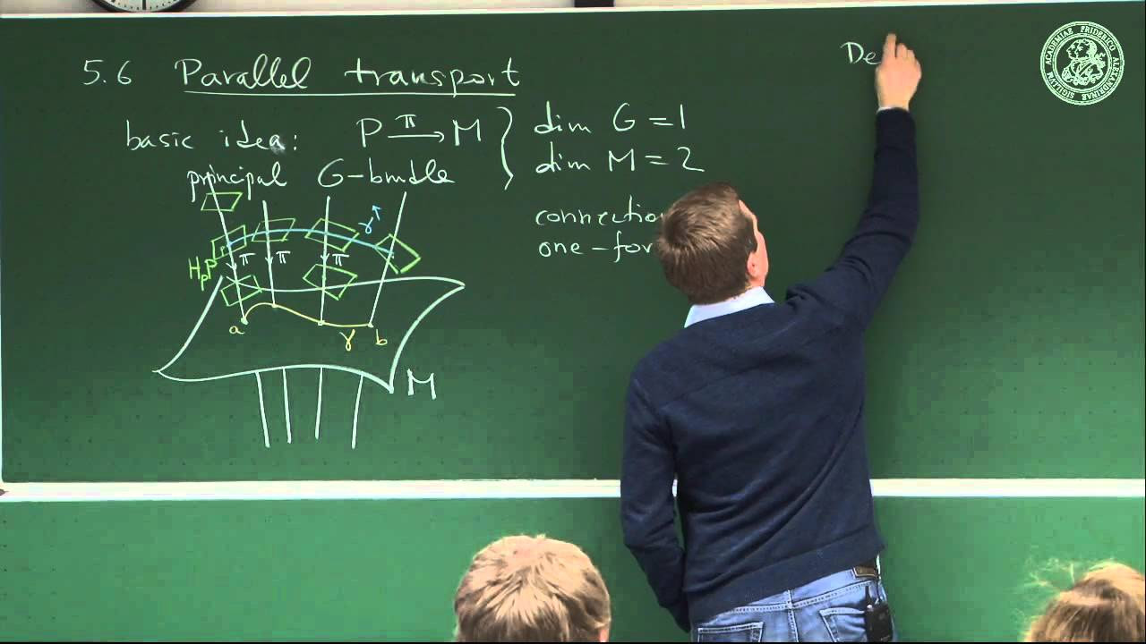
📚 Introduction to Parallel Transport on a Sphere
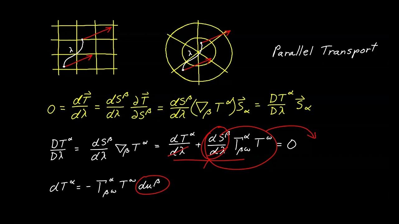
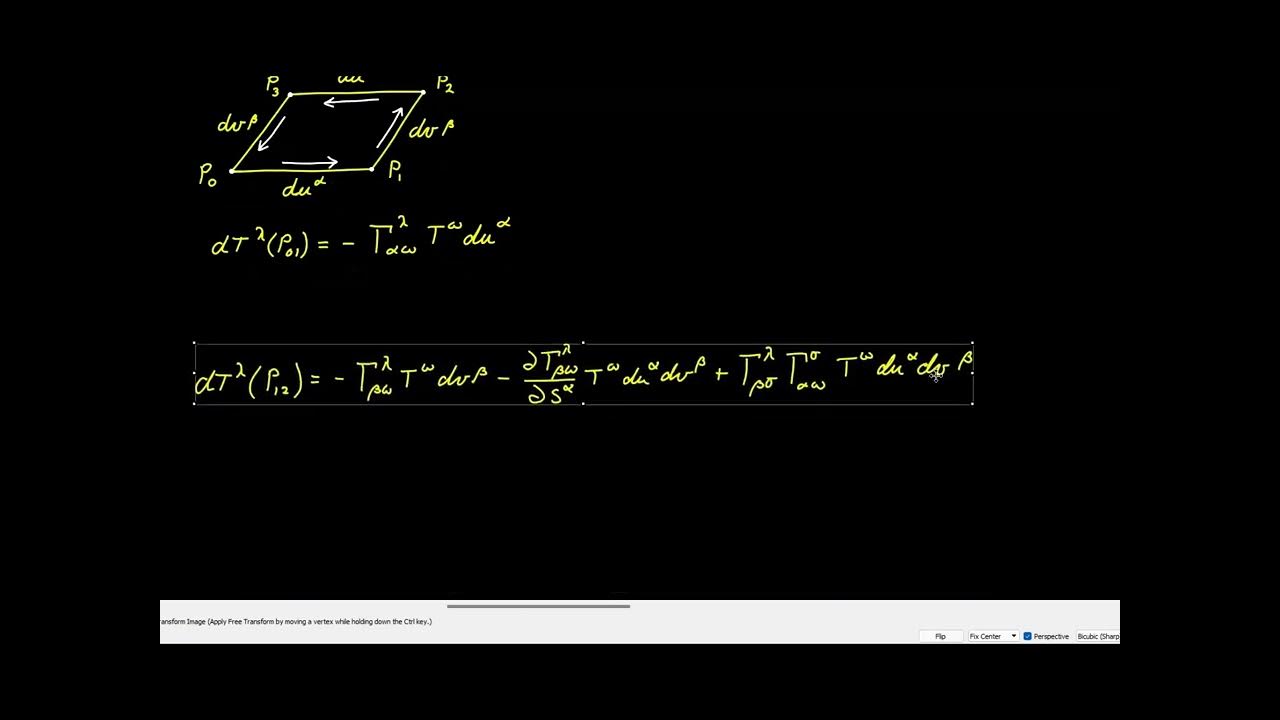
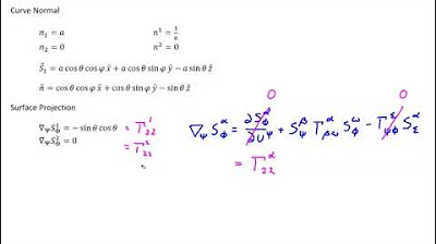
This paragraph introduces the topic of parallel transport in the context of tensor calculus, specifically focusing on a spherical surface. The video builds upon a previous demonstration, aiming to transport a vector T along a circle embedded in a sphere. The explanation begins with recalling the expression for parallel transport and emphasizes the importance of the derivative of the surface coordinates with respect to the parameter Phi. It is noted that since Theta is constant for the circle, certain terms in the equation can be ignored, simplifying the process. The paragraph also revisits the Christoffel symbols derived in a previous video and sets the stage for solving a pair of coupled differential equations, which are key to understanding parallel transport.
🔍 Solving Differential Equations for Parallel Transport
The second paragraph delves into the process of solving the differential equations necessary for parallel transport. It explains the method of differentiating one equation with respect to Phi to express the derivative of T2 in terms of T1, and then substituting back into the other equation to eliminate T2. This results in a second-order ordinary differential equation for T1. The process is reversed to obtain a similar equation for T2. The solutions to these equations are identified as expressions for simple harmonic motion, which can be solved with the application of initial conditions. The paragraph concludes with the final expressions for T1 and T2, which are constants due to Theta being a constant, and introduces the concept of angular velocity represented by the cosine of Theta.
📈 Visualizing Parallel Transport and Its Properties
The final paragraph discusses the visualization of the parallel transport process using graphing software. It describes how the vector T, initially a unit vector pointing in the Y direction, changes as it is transported along the curve. The paragraph explains the observed rotation of the vector and clarifies that it is not the vector itself that is changing, but rather the direction of the curve. The vector adjusts to remain parallel to itself, constrained to the tangent plane of the sphere. The summary also includes a sanity check by setting Phi to zero to confirm the initial condition and calculating the dot product of T with itself to ensure it remains a unit vector throughout the transport process. The paragraph concludes with an exploration of how changing the value of Theta affects the parallel transport, particularly noting the behavior when Theta is 90 degrees, forming a geodesic where the vector does not require adjustment.
Mindmap
Keywords
💡Parallel Transport
💡Spherical Surface
💡Coordinate System
💡Derivative
💡Christoffel Symbols
💡Coupled Differential Equations
💡Simple Harmonic Motion
💡Initial Conditions
💡Unit Vector
💡Geodesic
💡Holonomy
Highlights
Introduction to a specific example of parallel transport in tensor calculus, building on a previous demo.
Exploration of the parallel transport of vector T along a circle embedded in a spherical surface.
Recalling the expression for parallel transport and its parameterization using coordinate value Phi.
Derivative analysis of surface coordinate values S1 and S2 with respect to Phi, revealing constants and zero values.
Simplification of the parallel transport expression by ignoring certain terms based on the derivative outcomes.
Expansion of the expression and substitution of the Christoffel symbols for a spherical surface.
Derivation of a pair of coupled differential equations involving T1 and T2.
Methodology for solving coupled differential equations by taking derivatives and substitution.
Identification of the solutions as expressions for simple harmonic motion.
Application of initial conditions to the solutions for T1 and T2 to satisfy the differential equations.
Formation of the vector T as a linear combination of T Alpha and the surface basis vectors S Alpha.
Direct substitution of derived values for T1, T2, S1, and S2 into the final expression for vector T.
Verification of the vector T's unit magnitude through a sanity check by setting Phi to zero.
Demonstration of the parallel transport process using graphing software to visualize vector T's behavior.
Observation of the vector's adjustment to remain parallel while moving along a non-geodesic curve.
Comparison of vector behavior on a geodesic (great circle) where no adjustment is needed.
Analysis of vector behavior when theta exceeds 90 degrees, leading to a reversal in turning direction.
Conclusion summarizing the visual representation of parallel transport and its implications for holonomy in the next video.
Transcripts
Browse More Related Video
Video 96 - Parallel Transport
Video 99 - Holonomy Part 2
Tensor Calculus 22: Riemann Curvature Tensor Geometric Meaning (Holonomy + Geodesic Deviation)
Tensor Calculus 18: Covariant Derivative (extrinsic) and Parallel Transport
Video 94 - Sample Embedded Curve
Parallel transport - Lec 23 - Frederic Schuller
5.0 / 5 (0 votes)
Thanks for rating: