Tensor Calculus 18: Covariant Derivative (extrinsic) and Parallel Transport
TLDRThis video delves into the concept of the covariant derivative for curved surfaces, contrasting it with the flat space derivative. It introduces parallel transport, a method for moving vectors on a surface while keeping them as constant as possible. Using a sphere as an example, the video explains the challenges of defining constant vector fields on curved surfaces and demonstrates how the covariant derivative, given by Christoffel symbols, helps find vector fields that mimic parallel transport. The script provides mathematical formulas and examples to illustrate these concepts, emphasizing their significance in differential geometry and physics.
Takeaways
- 📚 The video introduces the concept of the covariant derivative for curved surfaces, building upon the understanding of the covariant derivative in flat space presented in a previous video.
- 🌐 It explains that working with vector fields on curved surfaces is more complex than in flat space due to the need to account for the curvature's impact on vector comparison and transport.
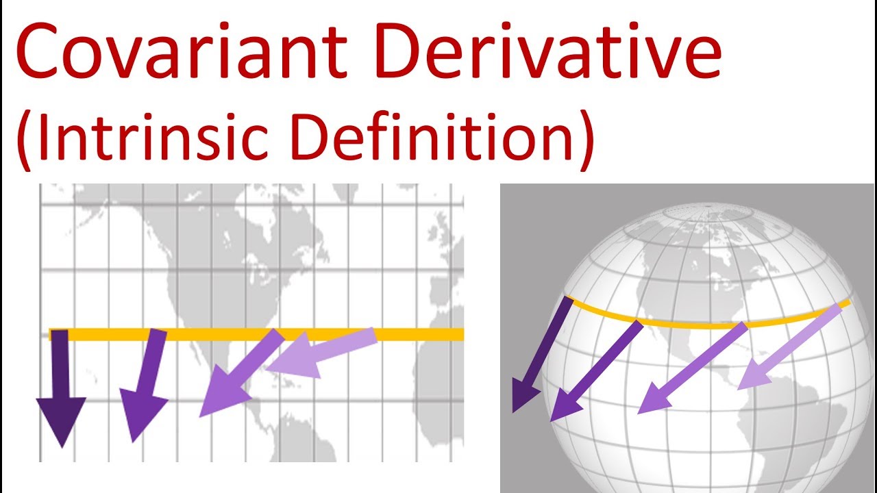
- 🔍 The script uses the sphere as a primary example to illustrate the challenges in comparing vectors on a curved surface, highlighting the issue of determining when two vectors are 'the same' on a sphere versus in flat space.
- 🚀 The concept of parallel transport is introduced as a method to move vectors around on a surface while keeping them as constant as possible, despite the inherent impossibility of maintaining a constant vector field on a curved surface.
- 🔄 The video demonstrates that parallel transport does not keep a vector constant when moved around a closed loop, due to the curvature of the surface, which results in a vector's direction changing upon return to the starting point.
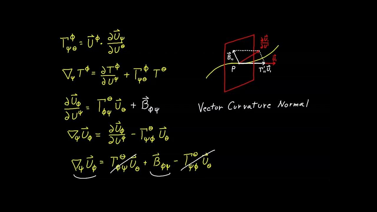
- 📉 The covariant derivative on curved surfaces is defined as the rate of change of a vector field in a given direction with the normal component of the rate of change subtracted, aiming to find vector fields that are as constant as possible through parallel transport.
- 📘 The script provides a detailed mathematical explanation of how to compute the covariant derivative on a sphere, including the need for Christoffel symbols, the second fundamental form, and the metric tensor.
- 📌 The video shows that the covariant derivative can be used to check if a vector field involves parallel transport by setting the covariant derivative to zero, which is the condition for parallel transport.
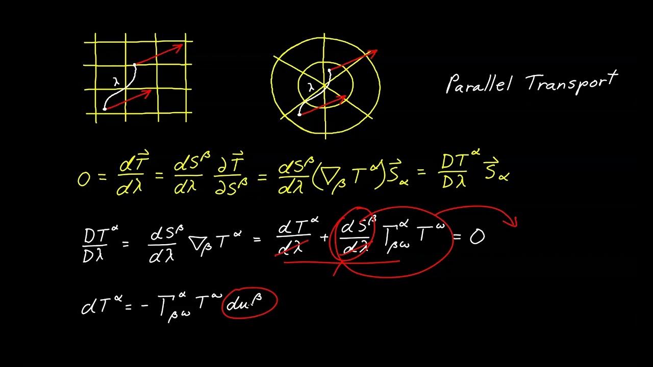
- 📐 An example is given of how to find a vector field resulting from parallel transporting an initial vector along a curve on a sphere, which involves solving differential equations with given initial conditions.
- 🔗 The script emphasizes that the covariant derivative is a tool that works for both curved and flat spaces, with the key difference being the subtraction of the normal component of the rate of change in curved spaces.
- 📊 The video concludes by reiterating that while it's impossible to define a truly constant vector field on a curved surface, the covariant derivative helps approximate this by finding vector fields that change as little as possible through parallel transport.
Q & A
What is the covariant derivative for flat space?
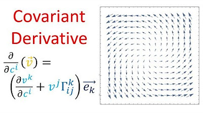
-In flat space, the covariant derivative of a vector field is essentially the ordinary derivative, where the product rule is applied to differentiate both the vector components and the basis vectors. It can also be expressed using Christoffel symbols, which represent the derivatives of the basis vectors as linear combinations of the basis vectors.
What is the purpose of parallel transport on a curved surface?
-Parallel transport is a method for moving vectors around on a surface in such a way that they remain as constant as possible from the perspective of an inhabitant of the surface. It is used to approximate what would be a constant vector field on a curved surface, which is inherently impossible to define.
Why is it not possible to define a constant vector field on a curved surface?
-A constant vector field on a curved surface is not possible because the concept of a vector remaining constant does not make sense from the perspective of someone living on the surface. Parallel transport is the closest approximation to maintaining a vector's constancy as one moves along a path on the surface.
What is the mathematical definition of the covariant derivative on curved surfaces?
-The covariant derivative on curved surfaces is defined as the derivative that gives the rate of change of a vector field V in some direction given by a vector W, with the normal component of the rate of change subtracted. It is represented by the symbol ∇_W V.
How does the covariant derivative relate to parallel transport?
-The covariant derivative is zero when a vector field V is being parallel transported in the direction W. This means that the vector is changing at a rate that is completely normal to the surface, indicating no change in the tangential direction.
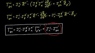
What are Christoffel symbols and how are they used in the context of the covariant derivative?
-Christoffel symbols are coefficients that describe how basis vectors change with respect to a coordinate system on a curved surface. They are used in the formula for the covariant derivative to account for the change in the basis vectors as one moves along the surface.
What is the significance of the normal component in the covariant derivative formula?
-The normal component in the covariant derivative formula represents the rate of change of the vector field that is perpendicular to the surface. Subtracting this component ensures that the derivative only accounts for changes within the tangent plane of the surface.
How do you calculate the Christoffel symbols for a given surface?
-To calculate the Christoffel symbols, one needs the tangent basis vectors, their derivatives, and the inverse metric tensor. By taking the dot product of the basis vector derivatives with the tangent vectors and using the metric tensor, one can derive the Christoffel symbols.
Can you provide an example of how to compute the covariant derivative on a sphere?
-An example of computing the covariant derivative on a sphere involves using the parametric formulas for the sphere's coordinates, calculating the tangent basis vectors and their derivatives, determining the metric and inverse metric tensors, and then applying these to the formula for the covariant derivative, which includes the Christoffel symbols.
What is the physical interpretation of a nonzero covariant derivative?
-A nonzero covariant derivative indicates that the rate of change of the vector field has a component in the tangent plane of the surface, meaning the vector is changing direction as it moves along the surface, which is consistent with the concept of parallel transport.
How does parallel transport affect the length of a vector?
-Parallel transport preserves the length of a vector. Even though the direction of the vector may change as it is transported along a curve on a surface, its magnitude remains constant.
Outlines
📚 Introduction to Covariant Derivative and Parallel Transport
The script introduces the concept of the covariant derivative for curved surfaces and parallel transport. It suggests watching a previous video for a foundation in flat space covariant derivatives. The covariant derivative on a flat surface is explained as an ordinary derivative with the product rule applied to both vector components and basis vectors. Christoffel symbols are introduced as a way to express basis vector derivatives. The video then transitions to the more complex topic of curved surfaces, using a sphere as an example, and highlights the difficulty of dealing with vector fields on such surfaces.
🌐 Understanding Vector Fields on Curved Surfaces
This paragraph delves into the challenges of working with vector fields on curved surfaces, contrasting constant and non-constant vector fields in flat space with those on a 2D sphere. It discusses the problem of comparing vectors on a sphere, illustrating the issue with the traditional method of sliding vectors to compare them due to the curvature of the surface. The concept of parallel transport is introduced as a method for moving vectors along a surface while keeping them as unchanged as possible, using the example of a journey from the North Pole to the equator on a sphere.
🔄 The Concept of Parallel Transport
The script explains the idea of parallel transport in more detail, describing it as a method to move vectors along a path on a surface while maintaining their direction as much as possible. It uses the analogy of a person on a planet to illustrate the concept and shows that parallel transport does not keep a vector constant when moved around a loop, due to the inherent curvature of the surface. The paragraph emphasizes that while parallel transport does not maintain a constant vector field, it is the best approximation for such a field on a curved surface.
📘 Mathematical Description of Parallel Transport
The paragraph focuses on the mathematical description of parallel transport, starting with the case of a curve on a sphere. It explains that the rate of change of a vector during parallel transport is always normal to the surface. The covariant derivative on curved surfaces is defined as the derivative that subtracts the normal component of the rate of change. The script provides a formula for the covariant derivative and explains its significance in finding vector fields that result from parallel transport, which are as constant as possible on a curved surface.
🔍 Calculating the Covariant Derivative on a Sphere
This section provides a detailed walkthrough of calculating the covariant derivative on a sphere, including the necessary steps to find the Christoffel symbols. It explains the process of obtaining the tangent basis vectors, their derivatives, and the inverse metric tensor. The paragraph also discusses how to use these components to compute the covariant derivative, highlighting that in flat space, the normal component of the rate of change is zero, which simplifies the calculation.
🌌 Examples of Covariant Derivatives and Parallel Transport on a Sphere
The script presents examples of calculating covariant derivatives and parallel transport on a sphere. It demonstrates how to find the covariant derivative of a vector field along a curve on the sphere and interpret the results. The examples include a vector field along the equator and another along a different curve with a non-zero covariant derivative, indicating a non-zero rate of change in the tangent plane. The paragraph concludes with the observation that a zero covariant derivative indicates parallel transport of the vector.
🔄 Parallel Transporting a Vector Field Along a Curve
This paragraph discusses the process of parallel transporting a vector along a curve on a sphere to generate a vector field. It provides an example starting with an initial vector and a curve, and then setting the covariant derivative of the vector field to zero to enforce parallel transport. The script solves the resulting differential equations to find the components of the vector field, illustrating how the vector field twists as it is transported along the curve due to the curve not being a great circle.
📈 Conclusion on Covariant Derivatives and Parallel Transport
The final paragraph summarizes the key points of the video, emphasizing the impossibility of defining a constant vector field on a curved surface and the role of parallel transport as the best approximation for such a field. It reiterates the definition of the covariant derivative as a tool for finding vector fields that are as constant as possible on a curved surface and highlights that when the covariant derivative is zero, the vector is being parallel transported. The script also notes that the covariant derivative works for both curved and flat spaces, with the normal component of the rate of change being zero in the latter.
Mindmap
Keywords
💡Covariant Derivative
💡Parallel Transport
💡Flat Space
💡Christoffel Symbols
💡Basis Vectors
💡Tangent Plane
💡Vector Field
💡Curvature
💡Geodesics
💡Metric Tensor
💡Second Fundamental Form
Highlights
Introduction to the covariant derivative for curved surfaces and its relation to parallel transport.
Recommendation to watch previous video on covariant derivative in flat space for foundational understanding.
Explanation of the covariant derivative in flat space using the product rule and Christoffel symbols.
Demonstration of the difference between handling vector fields in flat space versus curved surfaces.
The concept of parallel transport as a method for comparing vectors on a curved surface.
Illustration of the problem with traditional vector comparison methods on a sphere.
The impossibility of defining a constant vector field on a curved surface from a local perspective.
Introduction of the mathematical description of parallel transport and its limitations.
Visual explanation of the covariant derivative on a curve and its relation to normal vectors.
The covariant derivative defined as the derivative with the normal component subtracted.
Example of calculating the covariant derivative on a sphere with a specific vector field.
Description of the process to compute the Christoffel symbols necessary for the covariant derivative.
Detailed calculation of the Christoffel symbols for a sphere using the metric tensor.
Example of a vector field along the equator of a sphere and its covariant derivative.
Demonstration of parallel transport along a curve and the resulting vector field.
Solving differential equations to find a vector field that represents parallel transport.
Discussion on how parallel transport affects the direction and length of a vector field on a sphere.
Summary emphasizing the covariant derivative as a tool for finding parallel transported vector fields.
Transcripts
5.0 / 5 (0 votes)
Thanks for rating: