Video 94 - Sample Embedded Curve
TLDRThis video script from a tensor calculus series explores the concept of a curve embedded in a spherical surface, specifically a circle at an angle theta from the north pole. It delves into the mathematical framework required to describe such a curve, including the shift tensor, covariant and contravariant basis vectors, and the curvature properties. The script also explains how to calculate the geodesic curvature tensor and the vector curvature normal, ultimately demonstrating the decomposition of the vector curvature normal into surface and normal projections. The video concludes with a graphical demonstration of these concepts, providing a visual understanding of the curvature components and the special case of geodesic curves.
Takeaways
- 📚 The video discusses a specific example of a curve embedded in a spherical surface, illustrating tensor calculus concepts.
- 📈 The circle on the sphere is positioned at an angle theta from the north pole, with phi varying from 0 to 2π as the curve's coordinate.
- 🌐 The ambient coordinates for the curve are the spherical surface's coordinates, s1 and s2, requiring a parametrization in terms of phi.
- 🔍 The shift tensor is calculated with partial derivatives, resulting in s11 being 0 (due to theta being constant) and s21 being 1.
- 📉 The covariant basis vector for the curve is found to be equivalent to the surface's covariant basis vector s2, derived from previous analysis.
- 📏 The covariant metric tensor for the curve has a single component, determined by the dot product of the covariant basis vector with itself.
- 🔢 The contravariant metric tensor is the reciprocal of the covariant metric tensor, and the volume element is the square root of the covariant metric tensor's single component.
- 🔄 The inverse shift tensor is calculated, revealing that it simplifies to having components of 0 and 1, mirroring the shift tensor's structure.
- 🗺️ The Christoffel symbols for the curve are found to be zero, which simplifies the calculation of the vector curvature normal.
- 🧭 The vector curvature normal is derived from the partial derivative of the covariant basis vector, pointing in the direction of curvature.
- ⏱️ The magnitude of the vector curvature normal is the reciprocal of the curve's radius of curvature, confirmed by the relationship between the curve's radius and its curvature.
Q & A
What is the primary focus of the video on tensor calculus?
-The video focuses on demonstrating a specific example of a curve embedded in a surface, specifically a circle embedded in a spherical surface, and explores various tensor calculus concepts related to this curve.
What is the coordinate value for the curve in the video?
-The coordinate value for the curve is given by the value of phi, which varies from 0 to 2 pi, with u1 being equal to phi.
Why is the partial derivative of theta with respect to phi zero in the video?
-The partial derivative of theta with respect to phi is zero because theta is a constant value in this context, and the derivative of a constant is always zero.
What is the significance of the shift tensor in the context of the video?
-The shift tensor is significant as it represents the partial derivatives of the ambient coordinates with respect to the curve coordinates, which helps in understanding how the curve is embedded in the surface.
How is the covariant basis vector for the curve derived in the video?
-The covariant basis vector for the curve is derived using the relationship involving the shift tensor values, where it is found to be equal to the covariant basis vector s2 for the surface.
What is the role of the covariant metric tensor in the video?
-The covariant metric tensor is used to find the dot product of the covariant basis vector with itself, which helps in determining the curvature properties of the curve.
Why are the covariant and contravariant metric tensors reciprocals of each other for a curve?
-For a curve, the covariant metric tensor has only one component, and since there is only one dimension to invert, the contravariant metric tensor is simply the reciprocal of the covariant metric tensor.
How is the vector curvature normal calculated in the video?
-The vector curvature normal is calculated by taking the partial derivative of the covariant basis vector with respect to the curve coordinate, since the Christoffel symbols are found to be zero.
What does the magnitude of the vector curvature normal represent in the context of the video?
-The magnitude of the vector curvature normal represents the curvature value of the curve, which is the reciprocal of the radius of curvature of the embedded circle.
How does the video demonstrate the decomposition of the vector curvature normal into surface and normal components?
-The video demonstrates the decomposition by showing that the vector curvature normal can be expressed as the sum of the surface projection and the normal projection, which are derived from the geodesic curvature tensor and the surface curvature tensor, respectively.
What is the significance of the geodesic curvature tensor in the video?
-The geodesic curvature tensor represents the magnitude of the surface projection of the curve, which is a measure of how much the curvature of the path differs from that of a geodesic.
How does the video use graphing software to visually represent the concepts discussed?
-The video uses graphing software to visually demonstrate the curve, covariant basis vector, principal normal, surface normal, curve normal, vector curvature normal, surface projection, and normal projection, helping to clarify the relationships between these concepts.
What is the definition of a geodesic according to the video?
-A geodesic is defined as a curve that has no surface projection component and only a normal component, meaning it has the same curvature as the normal projection at every point along the curve.
Outlines
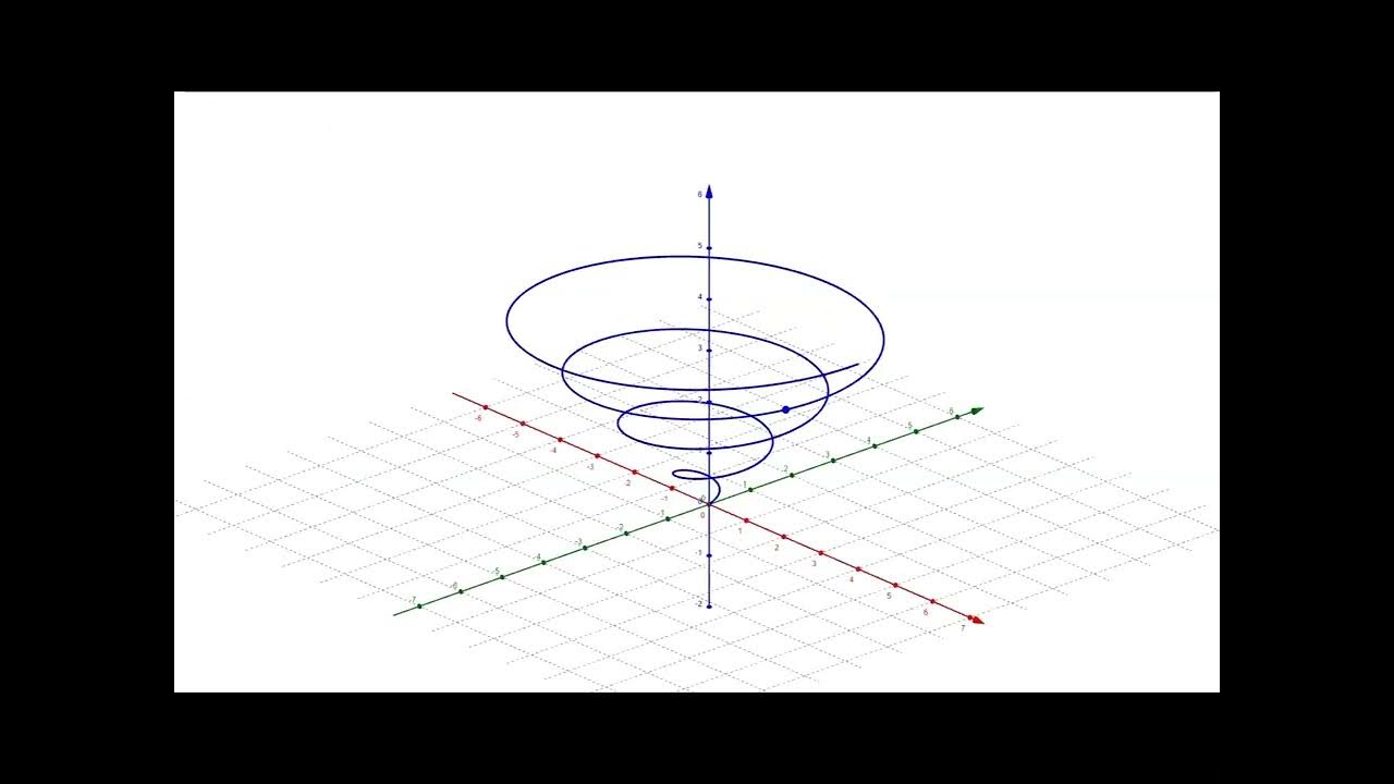
📚 Tensor Calculus: Curves on Surfaces
This paragraph introduces the topic of tensor calculus, specifically focusing on the example of a circle embedded in a spherical surface. The circle is positioned at a certain angle theta from the north pole, and the coordinate value for the curve is given by phi, which varies from 0 to 2 pi. The ambient space's coordinates are s1 and s2, which are the spherical surface's coordinates. The task is to find a parametrization of these coordinates as a function of phi, leading to the discovery of the shift tensor, which is essential for further calculations in the video.
🔍 Deriving the Shift Tensor and Covariant Basis Vector
The paragraph delves into the calculation of the shift tensor and covariant basis vector for the curve embedded in the spherical surface. The shift tensor is found by taking partial derivatives of the ambient coordinates with respect to the curve coordinates, resulting in s11 being 0 and s21 being 1. The covariant basis vector is then derived using the relationship between the shift tensor and the surface's covariant basis vector, which is obtained from previous analysis in video 61.
📈 Calculating the Covariant and Contravariant Metric Tensors
The focus of this paragraph is on finding the covariant metric tensor for the curve, which involves calculating the dot product of the covariant basis vector with itself. The result is a single component tensor, which also represents the determinant and volume element of the curve. The contravariant metric tensor is then derived as the reciprocal of the covariant metric tensor, and the contravariant basis vector is calculated using a specific relationship involving the covariant basis vector.
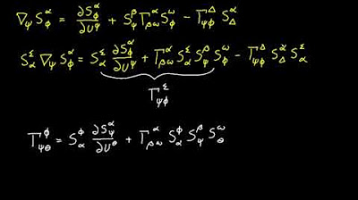
🧭 Exploring the Inverse Shift Tensor and Christoffel Symbols
The paragraph discusses the calculation of the inverse shift tensor, which involves expanding and simplifying expressions using the known values from the shift tensor and the surface's covariant metric tensor. The Christoffel symbols are also explored, with the conclusion that they are zero for the given curve, simplifying the calculation of the vector curvature normal.
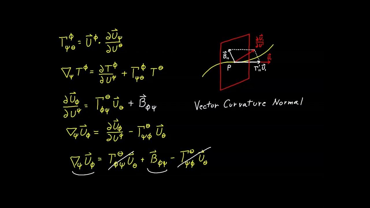
🌐 Vector Curvature Normal and Curvature Magnitude
This paragraph explains the process of finding the vector curvature normal by taking the partial derivative of the covariant basis vector with respect to the curve coordinate. The resulting vector is then used to calculate the curvature magnitude, which is shown to be the reciprocal of the curve's radius of curvature. The principal normal is derived by dividing the vector curvature normal by its magnitude, confirming its unit vector nature.
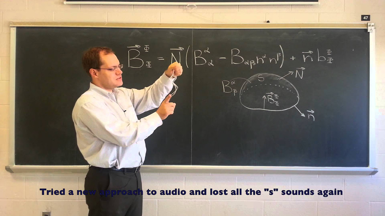
📉 Curve Normal and Surface Projection
The paragraph covers the derivation of the curve normal using the Levi-Civita symbols and the volume elements for both the surface and the curve. The components of the curve normal are calculated, and the vector itself is expressed in terms of the surface's covariant basis vectors. The surface projection is then explored, involving the calculation of the covariant derivative of the shift tensor and the Christoffel symbols, leading to the geodesic curvature tensor.
🌟 Visualizing Curvature Components and Geodesics
The final paragraph wraps up the video with a demonstration using graphing software to visually represent the concepts discussed in the previous paragraphs. It shows the decomposition of the vector curvature normal into surface and normal projections, and the significance of these components in understanding the curvature of the curve on the spherical surface. The special case of a geodesic curve, which has no surface projection and only a normal component, is highlighted, and the video concludes with a promise of further analysis of geodesic curves in the next installment.
Mindmap
Keywords
💡Curve
💡Spherical Surface
💡Shift Tensor
💡Covariant Basis Vector
💡Metric Tensor
💡Curvature
💡Principal Normal
💡Surface Projection
💡Normal Projection
💡Geodesic
Highlights
The video demonstrates a specific example of a curve embedded in a spherical surface, illustrating the concept of tensor calculus in a practical scenario.
The circle is located at an angle theta from the north pole, providing a suitable coordinate system for the curve.
The ambient coordinates for the curve are s1 and s2, which are the coordinates of the spherical surface.
A parametrization of the spherical surface coordinates as a function of phi is presented, with theta being a constant.
The shift tensor is derived, showing the relationship between the ambient coordinates and the curve coordinates.
The covariant basis vector for the curve is identified as being equal to the covariant basis vector s2 of the surface.
The covariant metric tensor is calculated, revealing its single component and determinant for the curve.
The contravariant metric tensor is found to be the reciprocal of the covariant metric tensor for the curve.
The contravariant basis vector is derived using the relationship between the covariant basis vector and the metric tensor.
The inverse shift tensor is calculated, showing its components and their relationship to the surface's metric tensor.
The Christoffel symbols are evaluated, resulting in a zero value for the curve due to its specific properties.
The vector curvature normal is derived, illustrating its components and relationship to the curve's geometry.
The magnitude of the vector curvature normal is calculated, providing the curvature value of the curve.
The principal normal is determined by dividing the vector curvature normal by its magnitude.
The curve normal is derived using the permutation symbol and the volume element of the surface.
The surface projection is calculated, demonstrating its components and their significance in the curve's behavior.
The geodesic curvature tensor is introduced, explaining its role in measuring the deviation from a geodesic path.
The normal projection is derived, showing its relationship to the surface normal and the curve's curvature.
A visual demonstration in graphing software ties together the theoretical concepts, providing a clear understanding of the curve's properties.
The significance of the surface and normal projections in understanding the curvature of a curve on a spherical surface is highlighted.
The concept of a geodesic curve is introduced, explaining its properties and the conditions under which it occurs.
Transcripts


5.0 / 5 (0 votes)
Thanks for rating: