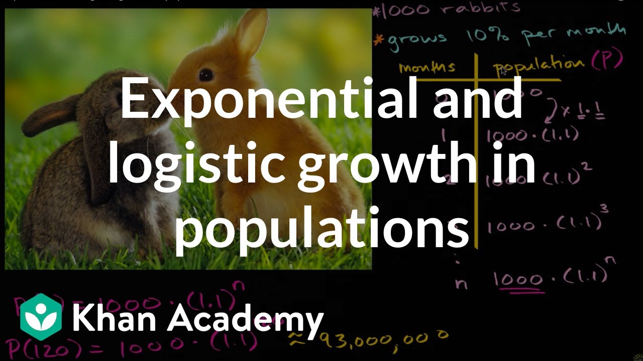
The Logistic Equation
TLDRThe video script discusses the concept of the logistic equation, a simple yet powerful model used to describe population growth that is influenced by competition. The presenter, Gilbert Strang, explains that while exponential growth would theoretically continue indefinitely, real-world factors such as competition for resources slow down growth, eventually leading to a stable population size known as the carrying capacity. The logistic equation is introduced as a way to model this phenomenon, and a mathematical trick is used to transform the nonlinear equation into a linear one, making it solvable. The resulting graph, known as a logistic or S-shaped curve, illustrates the transition from exponential growth to a stable state. The video also touches on the importance of understanding steady states and their stability in the context of differential equations, which is crucial for predicting outcomes in various real-world applications.
Takeaways
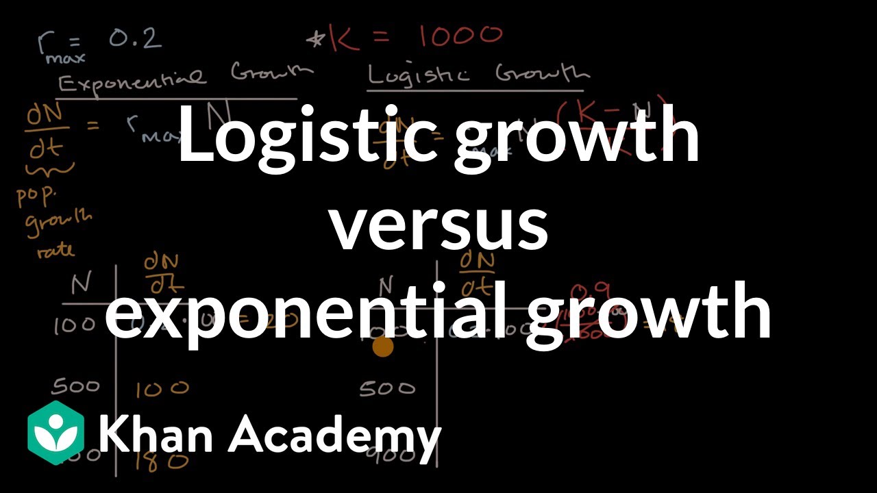
- 📈 The logistic equation is a simple model to describe population growth that is initially exponential but slows down due to competition among individuals.
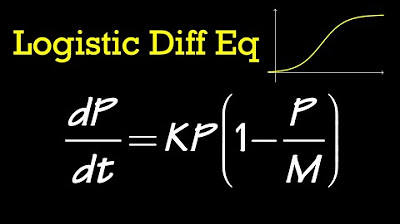
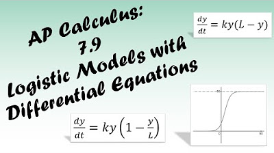
- 🌱 The growth rate is represented by the differential equation dy/dt = ay - by^2, where 'a' is the growth rate and 'b' is the competition factor.
- ✅ The logistic equation can be solved using a clever substitution method, introducing a new variable 'z' as 1/y, which transforms the equation into a linear form.
- 🔄 By solving for 'z', we find that dz/dt = -az + a constant, leading to an exponential solution for 'z' and subsequently for 'y'.
- 🌟 The solution to the logistic equation is often referred to as a logistic curve, S curve, or Sigmoidal curve, due to its S-shaped graph.
- 📉 The logistic curve approaches a limit, known as the carrying capacity (a/b), which represents the maximum population size that the environment can sustain.
- 🔴 The steady state y = 0 is unstable, meaning that a small population will grow exponentially until the competition term begins to slow the growth.
- 🟢 The steady state y = a/b is stable, as populations near this value will tend to stay close to it due to the balancing effects of growth and competition.
- 🌐 The logistic model, while simple, provides insight into how competition can regulate population growth and lead to a stable equilibrium.
- 📚 The concept of steady states and their stability is crucial for understanding more complex differential equations and their applications in various fields.
- ⏳ As time goes to infinity, the population growth asymptotically approaches the carrying capacity, and the exponential term in the solution diminishes.
Q & A
What is the simplest form of a nonlinear equation that describes population growth with competition?
-The simplest form of a nonlinear equation that describes population growth with competition is the logistic equation, which is dy/dt = ay - by^2, where 'a' represents the growth rate and 'b' represents the competition effect.
How does the logistic equation differ from an exponential growth model?
-The logistic equation differs from an exponential growth model by including a quadratic term (-y^2) that accounts for competition or limiting factors, which slows down the growth as the population size increases.
What is the trick used to transform the logistic equation into a linear equation?
-The trick is to introduce a new variable z = 1/y, which when substituted into the logistic equation, results in a linear equation for z in terms of time.
What is the significance of the term 'steady state' in the context of differential equations?
-A 'steady state' in differential equations refers to a condition where the derivative is zero, meaning the rate of change is zero and the system is in a stable, unchanging condition.
What are the two steady states for the logistic equation?
-The two steady states for the logistic equation are y = 0 (no population) and y = a/b (the carrying capacity where growth stops due to competition).
Why is the logistic curve also referred to as an S curve or a Sigmoidal curve?
-The logistic curve is referred to as an S curve or a Sigmoidal curve because its shape resembles the letter 'S', particularly when graphed, showing an initial rapid growth that slows down and levels off as it approaches the carrying capacity.
What is the term for the limiting population size in the logistic equation?
-The term for the limiting population size in the logistic equation is the carrying capacity, denoted as a/b.
How does the logistic equation model the effect of competition on population growth?
-The logistic equation models the effect of competition on population growth through the term -by^2, which represents the number of interactions among individuals that slow down the growth rate as the population size increases.
What does the solution to the logistic equation approach as time goes to infinity?
-As time goes to infinity, the solution to the logistic equation approaches the carrying capacity, a/b, which is the maximum sustainable population size in the presence of competition.
Why is the steady state y = 0 considered unstable in the logistic equation?
-The steady state y = 0 is considered unstable because any small increase in population from zero will lead to exponential growth, causing the system to move away from this state.
How does the logistic equation help in understanding the concept of 'blowing up' or 'settling down' in dynamic systems?
-The logistic equation helps in understanding these concepts by illustrating how different initial conditions can lead to different outcomes. If the system starts near y = 0, it 'blows up' or grows exponentially, while if it starts near y = a/b, it 'settles down' or stabilizes at the carrying capacity.
Outlines
📚 Introduction to Nonlinear Logistic Equation
The first paragraph introduces a simple nonlinear equation, known as the logistic equation, which models population growth with a competition factor. The equation is dy/dt = ay - by^2, where 'a' is the growth rate and 'b' represents the competition. Initially, the population grows exponentially (dy/dt = ay), but as it becomes large, competition slows the growth. The speaker uses a mathematical trick by introducing a new variable 'z' as 1/y, which transforms the logistic equation into a linear one, allowing for an easier solution. The solution involves exponential functions and highlights two key steady states: y=0 (no population) and y=a/b (stable population size where growth stops).
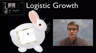
📈 The Logistic Growth Curve and Steady States
The second paragraph delves into the logistic growth curve, illustrating how population growth is initially exponential but slows down due to competition, eventually approaching a limit a/b. The speaker describes the curve as an 'S curve' or 'Sigmoidal curve' due to its shape. The concept of steady states is emphasized; these are values of y where the derivative is zero, indicating no change in the population size. Two steady states are identified: y=0, which is unstable (population will grow if starting near it), and y=a/b, which is stable (population will remain near this value). The paragraph also discusses the implications of these steady states in terms of population dynamics.
🔍 Stability of Steady States in Population Models
The third paragraph focuses on the stability of the steady states in the logistic equation. It distinguishes between unstable and stable steady states, noting that the population will rapidly grow away from y=0 (unstable), but will tend to stay near y=a/b (stable). The speaker mentions that the logistic equation serves as an example for a broader class of differential equations of the form dy/dt = f(y), where the stability of steady states is a critical aspect for practical applications. The paragraph concludes with a teaser for the next video, which will explore these types of equations further, particularly focusing on determining whether steady states lead to acceptable outcomes or catastrophic growth.
Mindmap
Keywords
💡Nonlinear Equation
💡Exponential Growth
💡Logistic Equation
💡Competition
💡Steady State
💡Carrying Capacity
💡Derivative
💡Sigmoidal Curve
💡Initial Value
💡Unstable Steady State
💡Stable Steady State
Highlights
Introduction to a simple nonlinear equation representing population growth with competition.
The logistic equation is presented as a model for population growth with a carrying capacity.
A trick is introduced to transform the logistic equation into a linear equation by using a substitution method.
The substitution involves a new variable z = 1/y, which simplifies the equation for analysis.
Derivation of the logistic equation's solution using the transformed linear equation.
The solution to the logistic equation is expressed in terms of exponential functions.
The logistic curve, also known as the S curve or Sigmoidal curve, is described and its significance is highlighted.
Explanation of the steady states in the logistic equation and their stability or instability.
The concept of carrying capacity (a/b) as a limiting factor for population growth is discussed.
Graphical representation of how the logistic curve approaches the carrying capacity over time.
The logistic equation's steady states are identified as y = 0 and y = a/b, representing no population and a balanced population respectively.
The importance of initial conditions on the behavior of the population growth is emphasized.
The logistic equation is used as an example to discuss the general problem of differential equations of the form dy/dt = f(y).
Differentiating between stable and unstable steady states in the context of population dynamics.
The implications of the logistic model for understanding real-world population growth and its limitations.
The logistic equation is presented as a starting point for more complex models that can account for additional factors like harvesting.
The video concludes with a teaser for the next video, which will delve into a more systematic approach to solving differential equations of the form dy/dt = f(y).
Transcripts
Browse More Related Video
5.0 / 5 (0 votes)
Thanks for rating: