AP Calculus BC Lesson 7.9
TLDRThis lesson delves into logistic growth and logistic differential equations, contrasting them with exponential growth. It explains that logistic growth models an S-shaped curve, where growth starts exponentially but levels off as it approaches the carrying capacity (L). The general solution to logistic differential equations is presented, highlighting that K is the growth constant and L is the limit as time approaches infinity. The lesson also discusses the point of inflection and maximum growth rate at L/2. Various examples, such as disease spread and population dynamics, illustrate the application of logistic models. The video concludes with problem-solving exercises that apply these concepts to real-world scenarios.
Takeaways
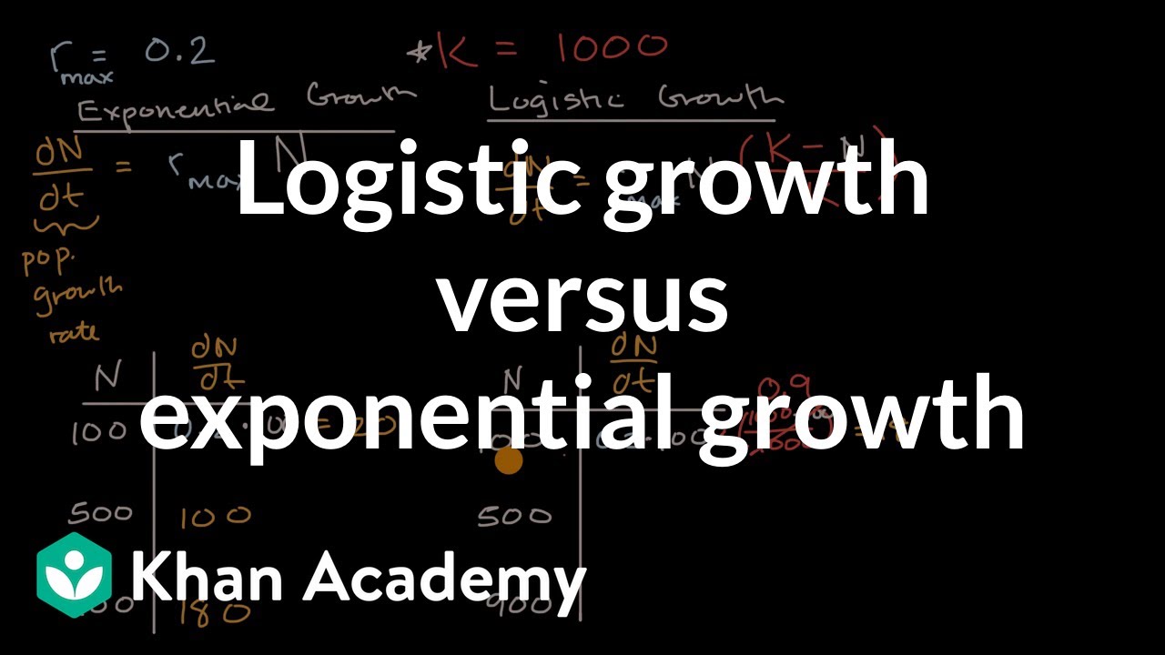
- 📈 The concept of logistic growth and logistic differential equations is introduced as a special case in basic calculus, distinct from exponential growth.
- 🔧 The general logistic growth model is represented by the differential equations dy/dt = k*y*(L - y) or dy/dt = k*y*(1 - y/L), where k and L are constants, and y is the dependent variable.
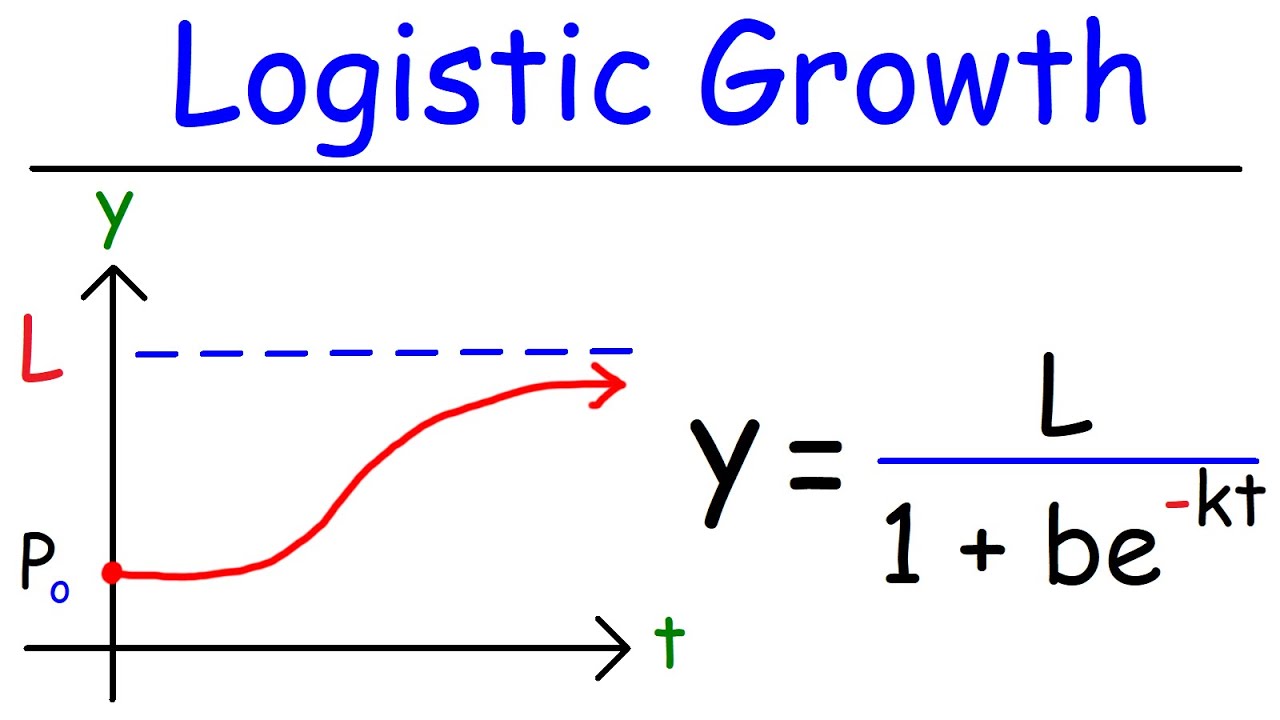
- 🌐 The general solution to logistic differential equations is y = L/(1 + Ce^(-kt)), which is not typically memorized for exams but is important for understanding the model.
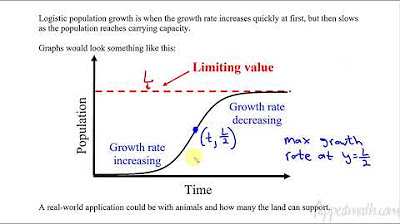
- 📊 Logistic growth models are characterized by an initial exponential-like growth that levels off as the carrying capacity (L) is approached, forming an S-shaped or sigmoid curve.
- 🔄 The carrying capacity (L) is the maximum value that the dependent variable (y) can approach as time (t) goes to infinity, and it represents the limit of growth.
- 📶 The derivative of y with respect to t (dy/dt) approaches zero as y approaches the carrying capacity, indicating a slowdown in growth rate.
- 🤔 The function y(t) has an inflection point at y = L/2, where the graph changes from concave down to concave up, signifying the point of fastest growth.
- 📈 The maximum value of the derivative (dy/dt) occurs at y = L/2, indicating the fastest growth rate at half the carrying capacity.
- 🚫 The derivative (dy/dt) is zero when y equals zero or the carrying capacity (L), indicating no growth at these points.
- 🐠 Examples of logistic growth include the spread of diseases, population size, and the propagation of rumors, all of which can be modeled by an S-shaped curve.
- 📌 The ability to rearrange given logistic differential equations to match standard forms is crucial for solving problems related to logistic growth.
Q & A
What are the two types of special case differential equations covered in basic calculus?
-The two types of special case differential equations covered in basic calculus are exponential growth and logistic growth.
What is the general solution for the exponential growth differential equation?
-The general solution for the exponential growth differential equation is y = ce^(kt), where k is a constant and c is an arbitrary constant.
What are the two possible forms of the logistic growth differential equation?
-The two possible forms of the logistic growth differential equation are dy/dt = ky(L - y) and dy/dt = ky(1 - y/L).
What does the constant K represent in the logistic growth differential equation?
-In the logistic growth differential equation, the constant K represents the growth rate of the function.
What is the meaning of L in the context of logistic growth?
-In logistic growth, L represents the carrying capacity or limiting capacity, which is the maximum population size that the environment can sustain indefinitely.
How does the logistic growth model differ from the exponential growth model in terms of the behavior of the function?
-Unlike exponential growth, which continues to increase without bound, logistic growth starts with an initial phase of rapid increase similar to exponential growth but then slows down and eventually levels off as it approaches the carrying capacity.
What is the significance of the point of inflection in a logistic growth function?
-The point of inflection in a logistic growth function is where the function changes from concave down to concave up, or vice versa. It represents the point at which the function's rate of growth is the highest.
At what value of y does the derivative dy/dt have a maximum in a logistic growth function?
-The derivative dy/dt has a maximum at y = L/2, which is half of the carrying capacity.
When does the derivative dy/dt equal zero in the context of logistic growth?
-The derivative dy/dt equals zero when y equals 0 or when y equals L, which are the points where the function starts and reaches its carrying capacity, respectively.
How can logistic growth be applied in real-world scenarios?
-Logistic growth can be used to model scenarios such as the spread of diseases over time, population size changes over time, or the spread of information like rumors.
What is the carrying capacity of the giraffe population in the given example, and how does this relate to the differential equation?
-The carrying capacity of the giraffe population is 50. This relates to the differential equation as it is the value of L in the equation, indicating the maximum sustainable population size.
How can you determine the differential equation that models a given logistic growth graph?
-To determine the differential equation that models a given logistic growth graph, you identify the carrying capacity (L) from the graph and then use the standard logistic differential equation format with the appropriate values for K and L.
Outlines
📚 Introduction to Logistic Growth and Differential Equations
This paragraph introduces the concept of logistic growth and logistic differential equations as part of a calculus lesson. It contrasts logistic growth with exponential growth, which was covered in a previous lesson. The differential equation for exponential growth is presented, followed by two equivalent forms for logistic growth's differential equation. The general solution for logistic growth is provided, with emphasis on the fact that it's not a memorization point for the AP exam. The paragraph also includes a graphical representation of logistic growth, highlighting the S-shaped curve and the concept of carrying capacity. The derivative's behavior as time approaches infinity is discussed, as well as the point of inflection and where the growth rate is the fastest.
🧪 Examples of Logistic Growth Applications and Problem Solving
This paragraph delves into practical applications of logistic growth, such as modeling the spread of diseases, population size, and the propagation of rumors. It emphasizes the S-shaped curve that characterizes logistic growth. The paragraph presents a multiple-choice question related to the spread of influenza, guiding the listener through the process of identifying the carrying capacity and solving for the limit as time approaches infinity. Two additional examples involving shark and rabbit populations are used to illustrate how to manipulate the logistic differential equation into standard forms for easier analysis. The paragraph concludes with a problem involving the rabbit population, showing how to determine the carrying capacity and when the population is increasing or growing fastest.
🦒 Giraffe Population Dynamics and Logistic Equation Analysis
The focus of this paragraph is on analyzing a giraffe population's growth using a logistic differential equation. It explains how to identify the carrying capacity and the point at which the population grows fastest. The paragraph provides a step-by-step guide on how to rewrite the given differential equation into a standard format to facilitate problem-solving. It also addresses a question about the rate of growth of the giraffe population and how to determine the value of the population size at which the growth is fastest. The process involves factoring out constants and rearranging terms to match the logistic differential equation structure.
🥫 Bacterial Growth in a Petri Dish: Modeling with Logistic Equations
This paragraph presents a scenario where the growth of bacteria in a Petri dish is modeled using a logistic differential equation. It describes how to construct the equation given specific conditions, such as the carrying capacity of the dish and the rate of change of bacteria at a certain population size. The paragraph guides the listener through the process of plugging in values and solving for the unknown constant to arrive at the logistic differential equation that accurately represents the bacterial growth situation. A multiple-choice question is also solved, with the correct differential equation identified based on the given data and the carrying capacity of the Petri dish.
Mindmap
Keywords
💡Logistic Growth
💡Logistic Differential Equations
💡Carrying Capacity (L)
💡Growth Rate Constant (k)
💡Exponential Growth
💡S-shaped Curve
💡Point of Inflection
💡Derivative
💡Disease Spread
💡Population Dynamics
Highlights
Logistic growth and logistic differential equations are discussed as special cases in basic calculus.
The differential equation for exponential growth is dy/dt = k*y, with the general solution y = c*e^(kt).
Logistic growth is modeled by two equivalent differential equations: dy/dt = k*y*(L - y) and dy/dt = k*y*(1 - y/L).
The general solution for logistic growth differential equations is y = L/(1 + c*e^(-kt)), which may not be memorized for the AP exam.
In logistic growth models, K is a constant and L represents the carrying capacity or limiting capacity.
The limit of y as time T approaches infinity is the carrying capacity L.
The derivative dy/dt approaches zero as T approaches infinity, reflecting the graph's leveling off.
The function y = T has a point of inflection at y = L/2, changing from concave down to concave up.
The derivative has a maximum at y = L/2, indicating the fastest growth rate at half the carrying capacity.
The derivative dy/dt is zero when y equals zero or L, representing the start and end of growth.
Logistic growth can model the spread of diseases, population size, or the spread of rumors over time.
The logistic growth graph shows an S-shaped curve, starting with exponential growth and then leveling off.
Rearrange the given logistic differential equation to match one of the standard equations for problem-solving.
Examples include using logistic growth to model the spread of influenza, shark populations, and rabbit populations.
The carrying capacity can be found by analyzing the differential equation and its parameters.
The point of inflection and the maximum growth rate can be determined from the logistic differential equation.
The logistic growth model can be applied to various real-world scenarios, such as giraffe populations and bacteria growth in a Petri dish.
The rate of change in a logistic model can be used to determine the fastest growth point within the population's carrying capacity.
To find the logistic differential equation that models a situation, substitute given values into the standard format and solve for the unknown constant.
Transcripts

5.0 / 5 (0 votes)
Thanks for rating: