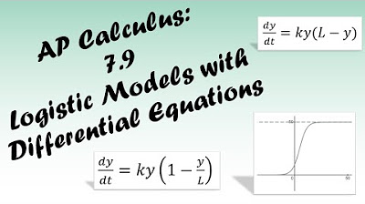
Logistic Differential Equation

RH Mathematics

6 Apr 202214:57

EducationalLearning

32 Likes 10 Comments

TLDRThis video script delves into the logistic differential equation, a model for constrained growth scenarios like population growth or disease spread. It introduces the equation's form, dp/dt = k*p*(1 - p/L), where 'p' is population, 'L' is carrying capacity, and 'k' is the growth rate constant. The S-shaped graph of logistic growth is highlighted, with the carrying capacity being the upper limit where growth levels off. Key points include the maximum growth rate occurring at half the carrying capacity and the presence of an inflection point at this point. The script also provides insights into the equation's application in real-world scenarios, such as infectious disease spread, and concludes with examples to solidify understanding.

Takeaways

📚 The logistic differential equation models scenarios like population growth or the spread of diseases, with a focus on constrained growth.
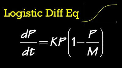
🔍 The standard form of the logistic differential equation is \( \frac{dp}{dt} = k \cdot p \cdot (1 - \frac{p}{L}) \), where \( p \) is the population, \( t \) is time, \( L \) is the carrying capacity, and \( k \) is a constant.
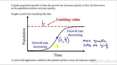
📈 The graph of the logistic equation typically has an S-shaped curve, indicating the growth rate slows as the population approaches the carrying capacity.
📉 If the initial population is above the carrying capacity, there will be a die-off, illustrating the importance of the carrying capacity in the model.
🧩 The carrying capacity \( L \) is proven to be the upper limit the population approaches as time goes to infinity.
📊 The maximum growth rate of the population occurs at half the carrying capacity, which is a crucial point for understanding the dynamics of logistic growth.
🔺 There is an inflection point in the logistic growth curve at half the carrying capacity, indicating a change in the concavity of the growth curve.
🌐 The logistic equation can be applied to various fields such as biology, environmental science, and human geography.
📝 For AP Calculus BC, understanding the form of the equation, the graph shape, the carrying capacity, and the maximum growth rate are essential.
📑 The solution to the logistic differential equation is not typically tested on AP Calculus exams but is important for a deeper understanding of the topic.
📚 Practice with logistic differential equations is encouraged to become familiar with different forms of the equation and their applications.

Q & A

What is a logistic differential equation typically used to model?
-A logistic differential equation is typically used to model scenarios involving constrained growth, such as the population of animals, the spread of an infectious disease, or any situation where growth is limited by a carrying capacity.
What does the variable 'p' represent in the logistic differential equation?
-'p' in the logistic differential equation represents the population at a given time.
What is the role of 't' in the logistic differential equation?
-'t' represents time in the logistic differential equation, but it is not a variable that is regularly used in the equation's solutions.
What is meant by 'carrying capacity' in the context of logistic growth?
-The 'carrying capacity' refers to the maximum population size that an environment can sustain indefinitely, given the food, habitat, water, and other necessities available in the environment.
What is the role of the constant 'k' in the logistic differential equation?
-'k' is a constant in the logistic differential equation that dictates how fast the growth is happening. It affects the rate at which the population increases or decreases.
What is the general shape of the graph for the solution of a logistic differential equation?
-The graph of the solution of a logistic differential equation typically has an S-shaped curve, indicating a slow start, rapid growth in the middle, and then leveling off as the population approaches the carrying capacity.
At what point does the maximum growth rate occur in a logistic growth scenario?
-The maximum growth rate in a logistic growth scenario occurs when the population is at half the carrying capacity.
What happens if the initial population is above the carrying capacity in a logistic growth model?
-If the initial population is above the carrying capacity, there will be a die-off, as the environment cannot support the population, leading to a decrease in population size.
How does the logistic differential equation relate to the spread of an infectious disease?
-In the context of infectious disease spread, the logistic differential equation can model how the disease spreads through a population. The growth rate of the disease is initially high when few people are infected, but as more people become immune or recover, the rate of new infections decreases.
What are the four key things one needs to know about the logistic differential equation for AP Calculus BC?
-For AP Calculus BC, one needs to know the form of the logistic differential equation (dp/dt = k * p * (l - p)), the general shape of the graph (S-shaped curve), the meaning of 'l' as the carrying capacity, and the fact that the maximum growth rate occurs when the population is half of the carrying capacity.

Outlines

00:00

📚 Introduction to Logistic Differential Equations

This paragraph introduces the logistic differential equation, which is used to model scenarios of constrained growth such as population growth or the spread of diseases. The logistic equation is presented in the form dp/dt = k * p * (1 - p/L), where p represents the population, t is time, L is the carrying capacity (an upper limit to growth), and k is a constant that dictates the growth rate. The paragraph emphasizes the importance of recognizing the logistic form of a differential equation and understanding its variables and parameters.

05:02

📈 Understanding the Logistic Growth Graph

The second paragraph delves into the graphical representation of the logistic differential equation, illustrating the characteristic S-shaped curve that represents growth constrained by the carrying capacity. It explains that the curve levels off as it approaches the carrying capacity, indicating a maximum sustainable population or growth rate. The paragraph also discusses the implications of starting with a population size above the carrying capacity, which would lead to a decline. Additionally, it touches on the mathematical proof that the carrying capacity L is indeed the upper limit of the growth, as the limit of p(t) as t approaches infinity is L.

10:02

📚 Key Facts about Logistic Differential Equations

This paragraph presents several key facts about logistic differential equations. It highlights that the maximum growth rate occurs at half the carrying capacity, which is a crucial piece of information for understanding how these equations model real-world scenarios. The paragraph also explains the concept of an inflection point, which occurs at the maximum growth rate, indicating a change in the concavity of the growth curve. The discussion includes the application of these concepts to the spread of infectious diseases, where the growth rate is initially low, peaks when half the population is infected, and then declines as it becomes harder to find new hosts.

📝 Applying Logistic Differential Equations in Problems

The final paragraph focuses on applying the knowledge of logistic differential equations to solve problems. It provides examples of how to identify the carrying capacity from an equation and how to calculate the growth rate at different population sizes. The paragraph also demonstrates how to find the value of k, the growth constant, using given information about the rate of population increase at a specific time. It concludes by emphasizing the importance of understanding the form of the equation, the shape of the graph, the concept of carrying capacity, and the maximum growth rate for success in AP Calculus BC exams.

Mindmap

Keywords

💡Logistic Differential Equation

A logistic differential equation is a mathematical model used to describe the growth of a population under conditions where the growth rate slows down as the population size approaches a certain limit. In the context of the video, it is used to model scenarios such as population growth of animals or the spread of an infectious disease, where growth is limited by factors like space or resources. The script mentions the equation's form: dp/dt = k*p*(1 - p/L), where 'k' is the growth rate constant, 'p' is the population size, and 'L' is the carrying capacity.

💡Population

Population refers to the total number of individuals in a species or group, which is the subject of growth in the logistic differential equation. The video script uses the term to discuss how the logistic equation models population growth, constrained by factors like space, as in the example of bacteria growing in a petri dish.

💡Carrying Capacity (L)

Carrying capacity, denoted as 'L' in the logistic equation, is the maximum population size that an environment can sustain indefinitely. The script explains that it represents the upper limit of population growth, such as the maximum number of bacteria that a petri dish can support, and it is a key parameter in the logistic model.

💡Exponential Growth

Exponential growth is a type of growth where the value of a quantity increases at a rate proportional to its current value. The video contrasts exponential growth with logistic growth, noting that while exponential growth continues without bound, logistic growth is self-limiting due to the carrying capacity.

💡Growth Rate

The growth rate in the context of the logistic equation is the speed at which the population increases, represented by the derivative dp/dt. The script explains that the growth rate is influenced by the current population size and the carrying capacity, and it peaks at half the carrying capacity.

💡S-shaped Curve

An S-shaped curve, or sigmoid curve, is the graphical representation of the logistic growth model. The video describes this curve as starting with a slow growth, accelerating to a midpoint, and then slowing down again as the population approaches the carrying capacity, eventually leveling off.

💡Inflection Point

An inflection point on a graph is a point where the curve changes its concavity. In the logistic model, the script mentions that there is a point of inflection where the growth rate is at its maximum, which corresponds to the population being at half the carrying capacity.

💡Derivative

In calculus, a derivative represents the rate of change of a function with respect to one of its variables. The video uses the term 'derivative' to describe the growth rate of the population, which is modeled by the logistic differential equation dp/dt.

💡Infectious Disease Spread

The script uses the spread of an infectious disease as an example of a scenario that can be modeled by the logistic differential equation. It explains how the growth rate of the disease slows as the population approaches the point where most individuals have been infected, illustrating the self-limiting nature of logistic growth.

💡Maximum Growth Rate

The maximum growth rate is the highest value that the growth rate of the population can reach. The video script states that this occurs when the population size is at half the carrying capacity, which is a critical point in understanding the dynamics of logistic growth.

💡AP Calculus

AP Calculus refers to a high school calculus course and exam that many students take to earn college credit. The video script mentions this to frame the discussion of logistic differential equations within the context of what students are expected to know for the AP exam.

Highlights

The video discusses the logistic differential equation, which models population growth or the spread of diseases under constraints.

The logistic differential equation is given by dp/dt = k * p * (1 - p/L), where p is population, t is time, L is carrying capacity, and k is a constant.

The carrying capacity, L, represents the maximum population size that the environment can sustain.

The logistic equation can be recognized in different forms, including dy/dx = number * y * (carrying capacity - y).

The graph of the logistic equation typically shows an S-shaped curve, indicating constrained growth.

The carrying capacity, L, is the limit of the population size as time approaches infinity.

The logistic growth curve levels off as it approaches the carrying capacity, unlike exponential growth.

If the initial population is above the carrying capacity, there will be a die-off, demonstrating the importance of starting conditions.

The solution to the logistic differential equation is derived and can be used to prove that L is the carrying capacity.

The maximum growth rate of the population occurs at half the carrying capacity, which is a key fact for understanding logistic growth.

A point of inflection on the logistic curve corresponds to the maximum growth rate, indicating a change in concavity.

The logistic differential equation can be applied to model the spread of infectious diseases, where growth rate is influenced by the number of susceptible hosts.

In the context of infectious diseases, the growth rate is low when few are infected and declines as the disease approaches saturation.

Four key aspects of the logistic differential equation for AP Calculus BC include its form, graph shape, carrying capacity, and maximum growth rate.

Examples are provided to illustrate how to identify and work with logistic differential equations in various contexts.

The video concludes with a summary of the essential knowledge required for AP Calculus BC regarding logistic differential equations.

Transcripts

Browse More Related Video

AP Calculus BC Lesson 7.9

Logistic Growth (Separable Differential Equations)

Logistic growth versus exponential growth | Ecology | AP Biology | Khan Academy

Logistic Growth

Calculus BC – 7.9 Logistic Models with Differential Equations

Logistic Differential Equation (general solution)