Statistics 101: Understanding Correlation
TLDRIn this educational video, the host, Brandon, introduces the concept of correlation in statistics, following a discussion on covariance. He explains the difference between covariance and correlation, emphasizing that while covariance indicates the direction of the linear relationship, correlation provides both direction and strength. Using scatterplots and real-world examples, he illustrates how to interpret these statistical measures, cautioning that correlation does not imply causation and is only applicable to linear relationships. The video also covers how to calculate the Pearson correlation coefficient and offers a rule of thumb for determining the existence of a relationship between variables.
Takeaways
- 😀 The speaker is recovering from a cold and apologizes for any potential difficulty in understanding.
- 🙌 Encouragement is given to viewers struggling in class to stay positive and remember their accomplishments thus far.
- 📚 The video is part of a series on basic statistics, focusing on bivariate relationships and the concept of correlation.
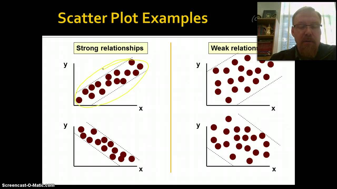
- 🔍 The importance of examining a scatterplot to understand the pattern of data points before calculating correlation is emphasized.
- 📈 Correlation measures both the direction and strength of a linear relationship between two variables, unlike covariance which only provides direction.
- 🔢 Correlation values range from -1 to 1, making it a standardized measure that is independent of the variables' scales.
- ⚠️ A reminder that correlation does not imply causation and that spurious correlations can occur without a real-life connection.
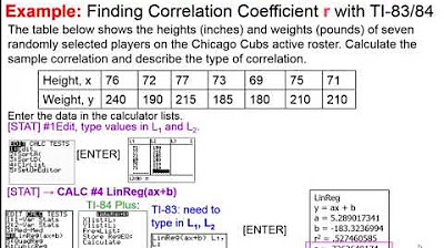
- 📉 The video provides an example of how to calculate the correlation coefficient using covariance and standard deviations.
- 📚 The formula for the Pearson correlation coefficient is explained, relating it to covariance and standard deviations.
- 📉 The video uses an example from Rising Hills Manufacturing to illustrate the calculation of the correlation coefficient.
- 📝 A rule of thumb is provided for determining if a relationship exists between two variables based on the correlation coefficient's value.
Q & A
What is the main topic of the video?
-The main topic of the video is understanding correlation in the context of basic statistics, particularly in relation to bivariate relationships.
Why does the speaker apologize at the beginning of the video?
-The speaker apologizes because they are recovering from a cold, which may affect the clarity of their voice during the video.
What encouragement does the speaker offer to viewers who might be struggling in a class?
-The speaker encourages viewers to stay positive, keep their heads up, and remember that they are smart and capable of overcoming temporary challenges with hard work, practice, and patience.
How does the speaker suggest viewers stay updated with their content?
-The speaker suggests that viewers follow them on YouTube and/or Twitter to be notified when new videos are uploaded.
What is the difference between covariance and correlation?
-Covariance provides the direction of the linear relationship between two variables, indicating whether they move together positively or negatively. Correlation, on the other hand, provides both the direction and the strength of the relationship, with values ranging from -1 to 1.
Why is it important to look at a scatterplot before calculating the correlation?
-Looking at a scatterplot is important to determine the pattern of the data points and ensure that they exhibit a linear relationship, as correlation is only applicable to linear relationships.
What does the speaker mean by 'correlation is not causation'?
-The speaker is emphasizing that even if two variables are correlated, it does not necessarily mean that one variable causes the other to occur. There could be a spurious correlation with no sensible real-life connection.
What is the formula for calculating the Pearson correlation coefficient?
-The Pearson correlation coefficient (r) is calculated as the covariance of the two variables divided by the product of their standard deviations.
How does the speaker describe the strength of a correlation?
-The strength of a correlation is described by how close the correlation coefficient is to -1 or 1, with values near these extremes indicating a strong relationship, and a value near 0 indicating a weak or non-existent relationship.
What is the rule of thumb for determining if a relationship exists between two variables based on the correlation coefficient?
-If the absolute value of the correlation coefficient is greater than 2 divided by the square root of the sample size, then a relationship is considered to exist between the two variables.
How does the speaker conclude the video?
-The speaker concludes by summarizing the key points about correlation, reminding viewers to stay positive and encouraging them to engage with the content by liking, sharing, and providing feedback.
Outlines
📚 Introduction to Basic Statistics and Encouragement
In the introduction, Brandon greets the audience and sets the stage for a basic statistics video, acknowledging his recent cold which might affect his voice clarity. He encourages viewers struggling with their studies to stay positive, reflecting on their past educational achievements and emphasizing the importance of hard work, practice, and patience. He invites viewers to follow him on YouTube and Twitter for updates on new content and asks for engagement through likes and shares to motivate content creation. The video aims to cover basic statistical concepts slowly and deliberately, ensuring understanding of both 'what' and 'why' in statistics.
🔍 Understanding Bivariate Relationships and Correlation
This paragraph delves into the topic of bivariate relationships, specifically focusing on correlation as a follow-up to previous discussions on covariance and scatterplots. Brandon uses a real-world example of the S&P 500 and Dow Jones Industrial Average monthly returns to illustrate the concept of a linear pattern in data points. He explains the importance of recognizing the shape of data distribution and the implications of positive linear relationships, particularly in the context of financial indices that are expected to measure the same underlying market performance. The paragraph also distinguishes between covariance, which indicates the direction of the relationship, and correlation, which provides both direction and strength of the relationship.
📊 The Difference Between Covariance and Correlation
Brandon clarifies the differences between covariance and correlation, noting that while covariance indicates the direction of the linear relationship between two variables, correlation goes further to express both the direction and the strength of that relationship. He points out that covariance lacks a fixed boundary and is dependent on the scale of the variables, whereas correlation is bounded between -1 and 1 and is independent of the variables' scale, making it a standardized measure. The paragraph also advises viewers to examine scatterplots before calculating correlations to ensure the relationship is linear and to remember that correlation does not imply causation.
📈 Correlation Patterns and Non-linear Relationships
This section discusses various patterns of correlation, including positive, negative, and zero linear relationships, and how they are represented visually in scatterplots. Brandon emphasizes that real-world data often falls between these extremes. He also introduces non-linear relationships, such as quadratic, exponential, and polynomial patterns, and stresses the importance of scatterplot analysis to determine the appropriateness of using correlation for a given dataset. The paragraph concludes with an example of calculating the correlation coefficient between the S&P 500 and Dow Jones, highlighting the strong positive correlation found.
🧑🏫 The Pearson Correlation Coefficient Formula
Brandon introduces the Pearson correlation coefficient, named after its inventor, and explains its formula in the context of covariance and standard deviations. He demonstrates how the correlation coefficient is derived from the covariance of two variables divided by the product of their standard deviations. The paragraph also touches on the concept that knowing any three of the variables (correlation coefficient, covariance, and the two standard deviations) allows one to calculate the fourth, which can be useful in various statistical applications.
🔢 Example Problem: Calculating the Correlation Coefficient
In this paragraph, an example problem from Rising Hills Manufacturing is presented to illustrate the calculation of the correlation coefficient between the number of workers and the number of tables produced. The data includes standard deviations and covariance, which are used to compute the correlation coefficient. The resulting strong positive correlation coefficient indicates a significant linear relationship between the number of workers and the production output. The paragraph also discusses the implications of this relationship and the difference between correlation and causation.
🤔 Rules of Thumb for Correlation and Final Thoughts
The final paragraph provides a rule of thumb for determining the existence of a relationship between two variables based on the correlation coefficient and sample size. It reiterates the key differences between covariance and correlation, emphasizing that correlation is a standardized measure applicable to linear relationships only. The paragraph concludes with words of encouragement for viewers facing academic challenges, an invitation to follow the channel for updates, and a reminder of the importance of the learning process over immediate results.
Mindmap
Keywords
💡Covariance
💡Correlation
💡Scatterplot
💡Linear Relationship
💡Standard Deviation
💡Pearson Correlation Coefficient
💡Statistical Significance
💡Causation
💡Spurious Correlation
💡Rule of Thumb
💡Bivariate Relationships
Highlights
Introduction to basic statistics series with a focus on bivariate relationships.
Apology for the speaker's cold and encouragement for students struggling in class.
Advice to stay positive and the acknowledgment of the viewers' educational accomplishments.
Encouragement to follow the speaker on YouTube and Twitter for updates on new videos.
Importance of understanding the basic concepts of statistics for newcomers.
Explanation of covariance and its role in understanding bivariate relationships.
Use of a scatterplot to visualize the relationship between the S&P 500 and Dow Jones Industrial Average.
Identification of a linear pattern in the data points of stock market returns.
Practical significance of the correlation between two stock indices measuring the same market performance.
Differentiation between covariance, which provides direction, and correlation, which provides both direction and strength.
Correlation's standardized nature allowing for comparison between variables measured in different units.
The importance of examining a scatterplot before calculating correlation to ensure linearity.
Clarification that correlation does not imply causation and the concept of spurious correlation.
Presentation of general correlation patterns and their interpretation on a scatterplot.
Example of calculating the correlation coefficient between the number of workers and tables produced.
Explanation of the Pearson correlation coefficient formula and its components.
Rule of thumb for determining the existence of a relationship based on the correlation coefficient.
Emphasis on the process of learning and the importance of continuous self-improvement.
Transcripts
Browse More Related Video


5.0 / 5 (0 votes)
Thanks for rating: