BusCalc 14.2 Partial Derivatives
TLDRThe transcript discusses the concept of partial derivatives in the context of multi-variable functions. It begins with an explanation of how solar panel efficiency can be modeled using latitude and cloud cover, introducing the variables and their impact on power output. The script then delves into evaluating multi-variable functions, contour lines, and traces, providing a mathematical exploration of these concepts. It continues with a detailed discussion on partial derivatives, illustrating how they extend the concept of derivatives to functions of multiple variables. The importance of the order of differentiation is highlighted, emphasizing that the order does not affect the outcome, a property known as Clairaut's theorem. Practical examples are given to demonstrate how to compute first and second partial derivatives, as well as mixed partials. The application of partial derivatives in understanding the rate of change and slope of tangent lines to surfaces is also explored. The summary concludes with an example involving the evaluation of a function involving natural logarithms and exponentials, showcasing the process of finding derivatives with respect to different variables and the utility of these mathematical tools in various real-world scenarios.
Takeaways
- 🌞 The power output of a solar panel is influenced by the latitude (theta) and the fraction of daytime that direct sunlight is obscured by clouds (C).
- 📐 At the equator (theta = 0), solar panels achieve maximum power output, while at the poles (theta = 90 degrees or π/2), the power output is minimal due to the tilt of the Earth away from the sun.
- ☁️ Cloud cover (C) significantly affects solar panel efficiency; areas with constant cloud cover, like Houston, would have a higher C value, reducing the power output compared to sunny areas like Phoenix.
- 🔢 The power output percent (P) can be calculated using the formula provided, which includes variables for latitude and cloud cover fraction.
- 🌐 Contour lines for solar panel power output can be determined by setting P to specific values and solving for theta and C, indicating regions of equal power output.
- 📉 At high latitudes (接近极点), solar panels may not receive any direct sunlight, especially when theta is around 81 degrees, which corresponds to a latitude near the poles.
- 🧮 Partial derivatives are used to find the slope of a tangent line to a surface at a specific point in a multivariable function, and they can be taken with respect to either variable while considering the other as constant.
- 🔄 The order of taking partial derivatives does not affect the result, a property known as Clairaut's theorem in multivariable calculus.
- 📈 First and second partial derivatives can provide information about the rate of change and curvature of a function's surface.
- 🔢 Evaluating partial derivatives at specific points gives the slope of the tangent line at those points in the respective direction of the derivative taken.
- 🚧 The concept of traces is introduced to find the behavior of a function when one of the variables is held constant, resulting in a single-variable function.
Q & A
What is the average electrical power of a solar panel approximated by?
-The average electrical power of a solar panel is approximated by an equation involving the percent of maximum power (p), the latitude in degrees (theta), and the fraction of the daytime that direct sunlight is obscured by clouds (C).
How does the latitude (theta) affect the power output of a solar panel?
-The power output of a solar panel decreases as the latitude increases, away from the equator. This is because the Earth's tilt results in less direct sunlight at higher latitudes.
What is the value of theta that corresponds to the equator?
-Theta equals zero corresponds to the equator, where direct sunlight is the most intense.
What does the variable C represent in the context of the solar panel power equation?
-C represents the fraction of the daytime that direct sunlight is obscured by clouds, affecting the solar panel's power output.
What is the power output percent (p) when the solar panel is installed at 30 degrees latitude with a cloud cover fraction (C) of 0.25?
-The power output percent (p) is approximately 75.5% of the maximum power that could be achieved under ideal conditions.
What does it mean to find the equation for the contour lines corresponding to p equal to 1?
-Finding the equation for the contour lines where p equals 1 means determining the conditions (latitude and cloud cover) where the solar panel operates at its maximum power output.
What is the trace of a function?
-The trace of a function is a single-variable function obtained by setting one of the independent variables to a constant, which allows us to see the relationship between the dependent variable and the remaining independent variable.
How is the concept of partial derivatives applied to multi-variable functions?
-Partial derivatives are used to find the rate of change of a multi-variable function with respect to one of its variables, while treating the other variables as constants.
What does the second partial derivative of a function represent?
-The second partial derivative of a function represents the rate of change of the first partial derivative with respect to the same variable, providing information about the curvature of the function in the direction of that variable.
Why is the order in which you take partial derivatives not important?
-The order is not important because of a property called Clairaut's Theorem, which states that the order of taking partial derivatives of a function with continuous second partial derivatives commutes, i.e., ∂²f/∂x∂y = ∂²f/∂y∂x.
What is the significance of evaluating a partial derivative at a specific point?
-Evaluating a partial derivative at a specific point provides the slope of the tangent line to the surface represented by the function at that point in the direction parallel to the axis with respect to which the derivative is taken.
Outlines
🔆 Solar Panel Power Calculation
The paragraph discusses the average electrical power output of a solar panel, which is influenced by the percent of maximum power (p), the latitude (theta), and the fraction of daytime with cloud cover (C). It explains that solar panels are more effective near the equator and less so near the poles due to the angle of sunlight. The power output percent (p) is calculated for a panel at 30 degrees latitude with 25% cloud cover, resulting in approximately 75.5% power output compared to equatorial conditions with no cloud cover.
📈 Contour Lines for Solar Power Efficiency
This section explores the equation for contour lines related to the power output (p) of a solar panel. It explains that when p equals 1, there is only a single point (theta equals 0 and C equals 0) where maximum power is achieved. For p equal to 0, the contour line is at theta equals 81 degrees, indicating no sunlight on the solar panel at or above this latitude. Lastly, for p equal to 0.5, any theta value can be chosen, and C can be solved accordingly, showing a range of possible combinations for half power output.
📊 Tracing Function for Cloud Cover Impact
The paragraph focuses on the trace of the function along the line where theta equals zero, representing the impact of cloud cover (C) on power output (p). It simplifies the power equation for this specific case and shows that as C varies from 0 to 1, p decreases from 1 to 0.5, illustrating the direct relationship between cloud cover and solar panel efficiency. Additionally, it presents a parabola representing the function when C equals 0, indicating the decrease in power output as latitude increases from the equator towards the poles.
🤔 Multi-Variable Functions and Their Derivatives
The content delves into multi-variable functions, specifically focusing on partial derivatives. It explains that partial derivatives extend the concept of derivatives to functions with more than one independent variable. The paragraph discusses how to take partial derivatives with respect to each variable while treating the others as constants. It also covers evaluating multi-variable functions, understanding contour lines, and tracing the function by setting one variable to a constant.
🧮 Evaluating Partial Derivatives
This section provides an example of evaluating partial derivatives. It demonstrates how to find the partial derivative of a function with respect to x at a specific point (1,2). The process involves differentiating each term of the function with respect to x, treating other variables as constants, and then evaluating the resulting expression at the given point.
🏞️ Visualizing Tangent Lines on Surfaces
The paragraph discusses the concept of tangent lines on surfaces represented by multi-variable functions. It explains that the partial derivative with respect to x represents the slope of the tangent line in the x direction, and similarly for the y direction. It uses a graph to illustrate how the slope of the tangent line changes depending on the direction of the line and the point on the surface.
🚴♀️ Application of Partial Derivatives in Real-Life Scenarios
This part of the script applies the concept of partial derivatives to a real-life scenario involving the effect of caffeine intake on a person's running speed. It uses a function to represent velocity and takes partial derivatives with respect to time (t) and caffeine intake (c) to analyze how these factors influence speed. The example shows how partial derivatives can be used to understand rates of change in different directions.
🔍 Higher Order Partial Derivatives and Notation
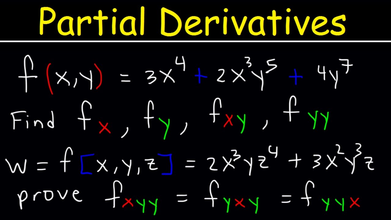
The paragraph introduces higher order partial derivatives and the associated notation. It explains how to denote first and second partial derivatives using subscripts and how to represent mixed partial derivatives. The content emphasizes the commutative property of partial derivatives, meaning the order in which they are taken does not affect the result.
🧱 Computing Second Derivatives of a Function
This section focuses on computing all first and second partial derivatives of a given function. It outlines the process of finding the partial derivatives with respect to x and y, as well as mixed partials. The paragraph demonstrates how to take these derivatives and emphasizes the importance of understanding the process for each term in the function.
📐 Evaluating a Specific Third Derivative
The content describes the process of evaluating a specific third derivative, g_xxx_y, at the point where x equals -1 and y equals 1. It explains the steps to find the necessary second derivatives and how to compute them. The paragraph also touches on the concept of a constant function as a result of differentiation.
🎢 Function Derivatives in a Dynamic System
This paragraph explores the concept of function derivatives in a dynamic system, represented by the variables h, x, and t. It demonstrates how to find mixed partial derivatives and single derivatives at a specific point. The example shows that certain mixed partial derivatives can be constant functions, independent of the variables' values.
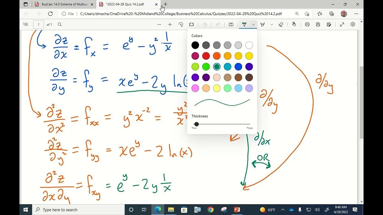
📘 Comprehensive Derivative Analysis
The final paragraph deals with finding all first and second derivatives of a function involving natural logarithm and linear terms. It explains the process of taking derivatives with respect to x and y, including the application of the chain rule and power rule. The content also covers the evaluation of mixed partial derivatives and the importance of checking work by taking different paths to the same derivative.
Mindmap
Keywords
💡Electrical Power
💡Latitude
💡Cloud Cover
💡Partial Derivatives
💡Contour Lines
💡Trace of a Function
💡Second-Order Partial Derivatives
💡Mixed Partials
💡Derivative Notation
💡Slope of a Tangent Line
💡Rates of Change
Highlights
The average electrical power of a solar panel can be estimated using a specific equation involving the percent of maximum power (p), latitude (theta), and cloud cover fraction (C).
At the equator (theta = 0), solar panels achieve the maximum power output due to the most direct sunlight.
At the poles (theta = 90 degrees or π/2), solar panels produce less power due to the tilt of the Earth away from the sun.
Cloud cover (C) significantly affects solar panel power output; areas with frequent cloud cover like Houston would have a higher C value, reducing power output.
For a solar panel installed at 30 degrees latitude with 25% cloud cover, the power output is approximately 75.5% of the maximum power.
Contour lines for p=1 indicate the only point of maximum power output, which is at the equator with no cloud cover (theta = 0, C = 0).
Contour lines for p=0 occur at high latitudes (theta = 81 degrees), indicating no sunlight on the solar panels at those locations.
The trace of the function along theta=0 shows a linear relationship between cloud cover fraction (C) and power output percent (p), ranging from full power (p=1) to 50% power (p=0.5).
Partial derivatives extend the concept of derivatives to multi-variable functions, providing the rate of change in a specific direction.
The partial derivative with respect to x (∂f/∂x) represents the slope of the tangent line to the surface in the x-direction.
Similarly, the partial derivative with respect to y (∂f/∂y) gives the slope of the tangent line in the y-direction.
The steepness of a surface at a point can be understood through the magnitude of its partial derivatives.
Second-order partial derivatives can be computed and are useful for understanding the curvature of a surface in multiple dimensions.
The order in which partial derivatives are taken does not affect the result, a property known as Clairaut's theorem.
Higher-order partial derivatives can be computed in various sequences to reach the same result, offering flexibility in calculations.
Evaluating partial derivatives at specific points provides insight into the behavior of a function at those points.
The effect of caffeine intake on speed can be modeled and analyzed using partial derivatives to understand how velocity changes with respect to caffeine intake.
Second-order partial derivatives can reveal the curvature and concavity of a function, important for understanding the function's behavior.
Transcripts


5.0 / 5 (0 votes)
Thanks for rating: