Introduction to Partial Derivatives (Calculus 3)
TLDRThis video script from Houston Mathprep offers a comprehensive introduction to partial derivatives, focusing on their conceptual understanding and calculation. It explains how to find the rate of change in two variable functions by considering one variable constant at a time. The script walks through the notation, including Leibniz and subscript notations, and provides step-by-step examples of first and second order partial derivatives, including mixed partials. It also highlights the typical equality of mixed second partial derivatives and the importance of notation order, concluding with an example involving a function of three variables.
Takeaways
- 📈 The script explains the concept of partial derivatives, focusing on how to find the rate of change in a 3D function along specific directions while holding other variables constant.
- 📚 It introduces two main directions for differentiation: along the x-axis with y held constant, and along the y-axis with x held constant, represented by ∂f/∂x and ∂f/∂y, respectively.
- 📝 The script clarifies the notation for partial derivatives, distinguishing between the Leibniz notation with a curly d and the subscript notation, e.g., f_x for ∂f/∂x.
- 🔍 The importance of partial derivatives is highlighted in functions of multiple variables, where ordinary derivatives are insufficient.
- 📐 Examples are provided to demonstrate the process of calculating partial derivatives for functions with two variables, using the chain rule and treating other variables as constants.
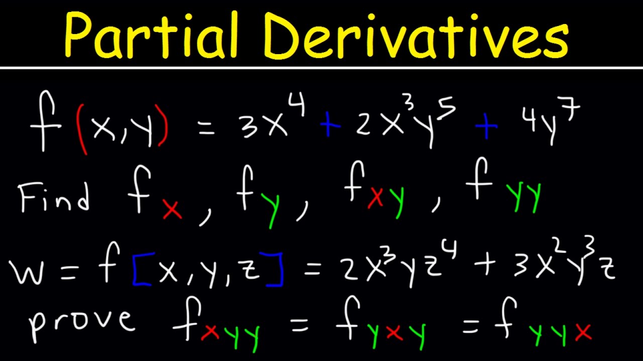
- 🔢 The transcript walks through the differentiation of specific functions, such as x^4y^2 + 5xy^3 + 3x - 9y + 2, step by step, applying the rules of differentiation to each term.
- 🌐 The concept of higher-order partial derivatives is introduced, including second partial derivatives and mixed partial derivatives, which can provide information about the concavity of a function in different directions.
- 🔄 The script points out that mixed second partial derivatives (f_xy and f_yx) are typically equal, a property that can be used for checking calculations.
- 📘 It also discusses the notation for mixed partial derivatives in the Leibniz notation, emphasizing the importance of reading the order from right to left.
- 📑 A final example involving a function of three variables (x, y, z) is given to illustrate the process of finding first partial derivatives with respect to each variable.
- 👍 The script concludes with a summary of the process and a wish for success in understanding partial derivatives, indicating a comprehensive coverage of the topic.
Q & A
What is a partial derivative?
-A partial derivative is a derivative that focuses on the rate of change of a function with respect to one variable while treating all other variables as constants.
How do you denote a partial derivative mathematically?
-A partial derivative can be denoted using the curly d notation, such as ∂f/∂x, or the subscript notation, such as f_x.
What is the difference between an ordinary derivative and a partial derivative?
-An ordinary derivative is used when the function is a function of a single variable, while a partial derivative is used when the function is a function of multiple variables.
How does the rate of change of a function in the x-direction differ from the rate of change in the y-direction at a point P?
-The rate of change in the x-direction at point P is found by considering a plane where y is constant and looking at the slope of the tangent line in the positive x-direction. Similarly, the rate of change in the y-direction is found by considering a plane where x is constant and looking at the slope of the tangent line in the positive y-direction.
What is the process of finding the partial derivative of a function with respect to x?
-To find the partial derivative of a function with respect to x, treat all other variables as constants and apply the standard derivative rules to the x terms in the function.
Can you provide an example of finding the partial derivative of a function with respect to x?
-For the function f(x, y) = x^4y^2 + 5xy^3 + 3x - 9y + 2, the partial derivative with respect to x, ∂f/∂x, is found by treating y as a constant and differentiating each term with respect to x, resulting in 4x^3y^2 + 5y^3 + 3.
What is the significance of mixed partial derivatives?
-Mixed partial derivatives, such as ∂²f/∂x∂y and ∂²f/∂y∂x, are used to find the rates of change in two different directions and can provide information about the concavity of a function in those directions.
Why are mixed partial derivatives often equal to each other?
-Mixed partial derivatives are often equal due to the Clairaut's theorem, which states that for functions of two variables that have continuous second partial derivatives, the order of differentiation does not matter.
How do you handle the chain rule when finding partial derivatives?
-When applying the chain rule for partial derivatives, you differentiate the outer function with respect to the inner function, treating all other variables as constants, and then multiply by the derivative of the inner function with respect to the variable of interest.
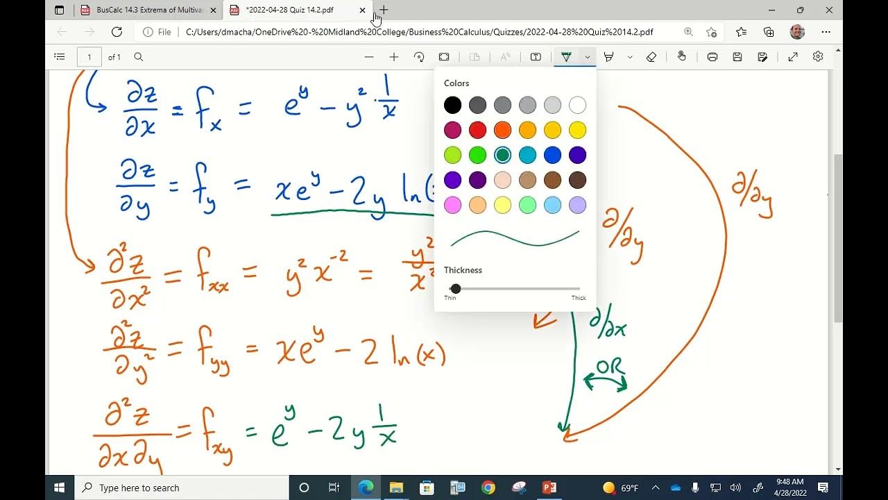
Can you give an example of a function involving a natural logarithm and how to find its partial derivatives?
-For the function f(x, y, z) = x * ln(yz), to find the partial derivative with respect to y, treat x and z as constants, differentiate the natural logarithm term with respect to y, resulting in f_y = xz/yz, which simplifies to x/y.
What is the importance of second order partial derivatives in analyzing a function?
-Second order partial derivatives, such as ∂²f/∂x² and ∂²f/∂y², can provide information about the concavity of a function in the x or y directions, which is crucial for understanding the function's behavior and for optimization problems.
Outlines
📚 Introduction to Partial Derivatives
The first paragraph introduces the concept of partial derivatives in the context of a 3D function graph. It explains how at a given point P, one can move uphill or downhill in various directions, and how the rate of change can be constant in some directions. The paragraph then explains the process of finding the rate of change in the x and y directions by holding one variable constant and using the tangent line to determine the slope. It introduces the notation for partial derivatives, distinguishing them from ordinary derivatives by the use of a curly d or subscript notation. The paragraph concludes with an example of finding partial derivatives for a function of x and y, emphasizing the rules of differentiation while treating the other variable as a constant.
🔍 Calculating Partial Derivatives
This paragraph delves deeper into the process of calculating partial derivatives with respect to x and y. It uses the same function from the previous example and demonstrates the steps to find the partial derivative with respect to y, treating x as a constant. The explanation includes applying the power rule and chain rule where necessary. The paragraph also covers shorthand notations for partial derivatives and provides a second example involving the sine function, which requires the use of the chain rule to find the partial derivatives with respect to both x and y.
🌐 Exploring Mixed Partial Derivatives and Higher Order Derivatives
The third paragraph discusses mixed partial derivatives and higher order partial derivatives. It explains that mixed partial derivatives are found by differentiating with respect to one variable and then the other, and notes that they are usually equal, a property that can be used for checking calculations. The paragraph also covers the calculation of second partial derivatives, both with respect to the same variable and mixed, using the function from the previous paragraph as an example. It highlights the importance of notation and the order of differentiation in Leibniz notation, especially when dealing with mixed partial derivatives.
📈 Second Derivatives and Their Applications
This paragraph continues the discussion on second derivatives, explaining their role in determining the concavity of a function in the x or y directions. It provides an example of a function with two variables and shows the process of finding all possible second partial derivatives, including mixed partial derivatives. The paragraph emphasizes the typical equality of mixed second partial derivatives and the importance of checking this equality as a validation of the calculations.
📘 Partial Derivatives in Functions of Three Variables
The final paragraph extends the concept of partial derivatives to functions of three variables, x, y, and z. It demonstrates how to calculate the first partial derivatives with respect to each variable, treating the others as constants. The example function involves a natural logarithm, and the paragraph shows the steps to find partial derivatives for each variable, including the application of the chain rule. The summary concludes with the final expressions for the partial derivatives of the given function.
Mindmap
Keywords
💡Partial Derivative
💡Rate of Change
💡Tangent Line
💡Leibniz Notation
💡Ordinary Derivative
💡Constant Multiple Rule
💡Chain Rule
💡Product Rule
💡Second Partial Derivatives
💡Mixed Partial Derivatives
💡Natural Logarithm
Highlights
Introduction to the concept of partial derivatives in 3D space focusing on the rate of change in specific directions at a point on a function.
Explanation of how to find the rate of change in the x-direction by treating y as a constant and vice versa.
Visual representation of the rate of change uphill, downhill, and constant height on a 3D function graph.
Differentiation between partial derivatives and ordinary derivatives based on the number of variables in a function.
Introduction of the Leibniz notation for partial derivatives using the curly d symbol.
Subscript notation as an alternative method to represent partial derivatives.
Demonstration of calculating partial derivatives for a function involving x and y using both Leibniz and subscript notations.
Application of derivative rules while treating the other variable as a constant in partial derivative calculations.
Example calculation of partial derivatives for a function with terms like x to the power of 4 times y squared.
Use of the chain rule in partial derivatives for functions involving trigonometric and exponential components.
Calculation of partial derivatives for a function with an exponential term e to the power of xy.
Product rule application in partial derivatives for functions that are products of variables.
Introduction to higher-order partial derivatives and their role in providing information about the concavity of functions.
Explanation of mixed partial derivatives and their significance in calculus.
Example of finding all possible second partial derivatives for a function of x and y.
Clarification on the equality of mixed second partial derivatives, fxy and fyx, in most cases.
Importance of notation order in Leibniz notation for mixed partial derivatives.
Final example involving a function of three variables, x, y, and z, demonstrating the calculation of partial derivatives with respect to each variable.
Conclusion and summary of key points regarding partial derivatives, including practical tips for students.
Transcripts


5.0 / 5 (0 votes)
Thanks for rating: