BusCalc 14.3 Extrema of Multivariable Functions
TLDRThe transcript details a comprehensive exploration of multi-variable calculus, focusing on finding and characterizing critical points of functions involving two independent variables, x and y. The speaker explains the process of calculating first and second partial derivatives with respect to each variable, emphasizing the importance of treating the other variable as a constant during these calculations. The concept of mixed partial derivatives is introduced, and the speaker clarifies that the order of differentiation does not affect the result. The video also delves into identifying and classifying critical points as maxima, minima, or saddle points using the second derivative test, which involves evaluating specific combinations of second derivatives at the critical points. The speaker illustrates the process with several examples, demonstrating how to solve systems of equations to find critical points and how to apply the second derivative test to determine their nature. The examples highlight various scenarios, including functions with maxima, minima, saddle points, and points where the second derivative test is inconclusive. The summary underscores the mathematical rigor and step-by-step approach necessary to understand and apply these concepts in calculus.
Takeaways
- 📘 Derivatives in multi-variable functions: For a function z = f(x, y), the first partial derivatives are ∂z/∂x and ∂z/∂y, considering y and x as constants respectively.
- 📙 Second partial derivatives: These include ∂²z/∂x², ∂²z/∂y², and the mixed partial ∂²z/∂x∂y, which does not depend on the order of differentiation.
- 📗 Treating variables as constants: When finding partial derivatives, treat the other variable as a constant.
- 📕 Critical points in single-variable functions: These are points where the first derivative is zero, and they can be classified as maxima, minima, or neither by using the second derivative.
- 📔 Characterizing critical points: Use the second derivative test to determine if a critical point is a maximum, minimum, or neither by checking if it's positive, negative, or zero.
- 📒 Extrema in multi-variable functions: Requires finding both first and second partial derivatives and using a determinant test (m-value) to classify critical points as maxima, minima, saddle points, or inconclusive.
- 📓 Saddle points: A special case in multi-variable functions where a point acts as a maximum in one direction and a minimum in another.
- 📔 Setting up systems of equations: To find critical points in functions of multiple variables, set the first partial derivatives equal to zero and solve the system of equations.
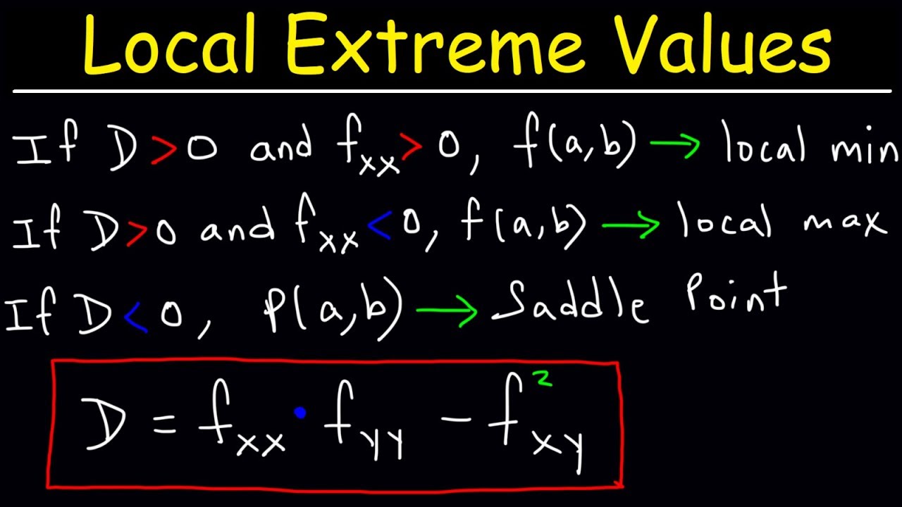
- 📒 m-Test for multi-variable functions: Use the formula m = (∂²z/∂x²)(∂²z/∂y²) - (∂²z/∂x∂y)² evaluated at the critical point to classify it.
- 📘 Positive m-value: If m > 0 and ∂²z/∂x² is negative, the critical point is a local maximum. If ∂²z/∂x² is positive, it's a local minimum.
- 📙 Negative m-value: If m < 0, the critical point is a saddle point. If m = 0, the test is inconclusive.
Q & A
What is a multi-variable function?
-A multi-variable function is a function that has more than one independent variable. In the context of the script, z is the dependent variable, and x and y are the independent variables.
What are the first partial derivatives?
-The first partial derivatives are the derivatives of the function z with respect to each of its independent variables, x and y. They represent the rate of change of z with respect to x and y while keeping the other variable constant.
How are second partial derivatives different from first partial derivatives?
-Second partial derivatives are derived by taking the derivative of the first partial derivatives. They represent the curvature or the rate of change of the rate of change of the function with respect to each independent variable and can indicate if a point on the function is a maximum, minimum, or saddle point.
What is a mixed partial derivative?
-A mixed partial derivative is a second derivative that is found by taking the partial derivative with respect to one variable and then taking another partial derivative with respect to the other variable (or vice versa). The order in which the derivatives are taken does not affect the result for well-behaved functions due to Clairaut's theorem.
What does it mean to 'pretend y is a constant' when taking the derivative with respect to x?
-When taking the derivative with respect to x, 'pretending y is a constant' means that you treat y as if it does not change when calculating the derivative. This allows you to focus solely on how the function changes with respect to x while holding y constant.
How does the process of finding extrema (maximums and minimums) for multi-variable functions differ from single-variable functions?
-For multi-variable functions, you find critical points by setting the first partial derivatives equal to zero. Then, you use the second partial derivatives and a test involving them (referred to as the 'm test' in the script) to determine if a critical point is a local maximum, minimum, saddle point, or inconclusive. For single-variable functions, you only need the first and second derivatives.
What is a saddle point?
-A saddle point is a critical point of a function where the function neither reaches a maximum nor a minimum. It is a point where the function has a zero first derivative but the second derivative test is inconclusive or indicates a 'saddle' shape in the function's contours.
How do you find the critical points of a function?
-To find the critical points of a function, you first calculate the first partial derivatives with respect to each independent variable. Then, you set these first partial derivatives equal to zero and solve for the variables to find the critical points.
What is the 'm test' used for?
-The 'm test' is used to characterize the critical points of a multi-variable function. It involves calculating a value 'm' using the second partial derivatives and the mixed partial derivative at the critical point. Depending on the sign of 'm' and the sign of the second derivative with respect to x, you can determine if the critical point is a maximum, minimum, saddle point, or inconclusive.
What is the significance of the second derivative being zero at a critical point?
-If the second derivative is zero at a critical point, it does not provide enough information to determine whether the point is a maximum, minimum, or saddle point. This situation is inconclusive, and further analysis is required to understand the nature of the critical point.
How can you use the process described in the script to check your work when finding derivatives?
-You can check your work by taking derivatives in different orders. For example, you can take the derivative with respect to x first and then y, or vice versa. If the mixed partial derivative is the same regardless of the order in which you take the derivatives, it confirms that your calculations are correct due to the property of continuity and Clairaut's theorem.
Outlines
📚 Introduction to Multi-variable Derivatives
The video begins with an explanation of finding first and second derivatives of a multi-variable function, specifically a function z dependent on variables x and y. The presenter clarifies the concept of partial derivatives with respect to x and y, and introduces the idea of mixed partial derivatives. The process of differentiating while treating one variable as constant is also discussed.
🧮 Derivation of Second Derivatives and Mixed Partials
This paragraph delves into the calculation of second derivatives with respect to x and y, as well as the mixed partial derivative. The presenter uses the power rule for differentiation and emphasizes the importance of treating the other variable as a constant. The concept of checking work by taking derivatives in different orders for mixed partials is also highlighted.
🔍 Identifying Critical Points and Extrema
The focus shifts to finding maximums and minimums, known as extrema, of functions. The presenter explains the process of determining critical points by setting the first derivative to zero and using the second derivative to identify if a point is a maximum, minimum, or neither. The concept of concavity is introduced to characterize the shape of the function around critical points.
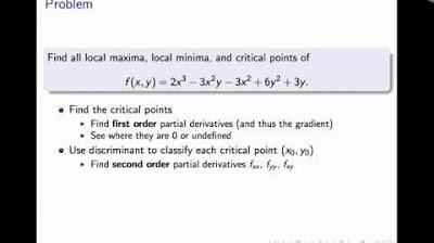
🔢 Example: Characterizing Critical Points
An example is provided to illustrate the process of finding and characterizing critical points of a function. The presenter shows how to find the first and second derivatives, set them to zero to find critical points, and then use the second derivative test to determine the nature of these points as maxima, minima, or neither.
📈 Multi-variable Function Analysis
The presenter discusses the analysis of multi-variable functions, introducing the concept of saddle points, which are unique to multi-variable functions. The video shows how to find and characterize critical points in these functions, including using second derivatives and a specific test to determine if a point is a saddle point, maximum, or minimum.
🤔 Dealing with Indeterminate Results
This part of the script addresses the situation where the second derivative test is inconclusive due to the second derivative being zero. The presenter explains that this does not provide enough information to determine if the point is a maximum, minimum, or saddle point, and further analysis is required.
📐 Solving Systems of Equations for Critical Points
The presenter demonstrates solving a system of two algebraic equations with two unknowns to find the critical points of a function. The process involves substitution and simplification to solve for the variables x and y, leading to the identification of multiple critical points.
📈 Characterizing Critical Points with the M Test
The M test is used to characterize the critical points found in the previous paragraph. The presenter calculates the value of M using second derivatives and the mixed partial derivative at the critical points. Different outcomes of the M test are discussed to determine if the points are maxima, minima, saddle points, or inconclusive.
🏞️ Visualizing Function Extrema with Graphing Calculator
The video concludes with a demonstration of using a graphing calculator to visualize the function's extrema. The presenter plots the function and identifies the locations of the saddle point and maximum value, confirming the results of the M test and providing a visual aid to understand the function's behavior.
Mindmap
Keywords
💡Derivative
💡Partial Derivative
💡Critical Points
💡Second Derivative Test
💡Saddle Point
💡Concave Up/Down
💡Multivariable Function
💡Mixed Partial Derivative
💡Optimization
💡Logarithm
💡Exponentiation
Highlights
The concept of dependent and independent variables in multi-variable functions is introduced, with z as the dependent variable and x and y as independent variables.
First partial derivatives are found by differentiating with respect to one variable while treating the other as a constant.
Second partial derivatives involve taking the derivative of the first partial derivative, again treating the other variable as constant during the process.
Mixed partial derivatives do not depend on the order of differentiation, a property that can be used to check work.
The process of finding extrema (maxima and minima) in single-variable functions is reviewed, emphasizing the role of first and second derivatives.
A new concept, saddle points, is introduced as a type of critical point unique to multi-variable functions.
The use of a second derivative test to classify critical points as maximums, minimums, or saddle points in multi-variable functions is explained.
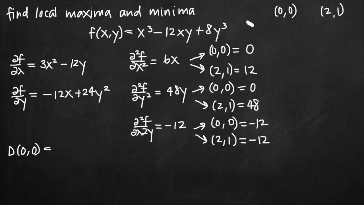
A step-by-step method for finding and characterizing critical points of a function is demonstrated through several examples.
The importance of setting first derivatives to zero to find critical points is underscored.
The calculation of an 'm' value from second derivatives is used to determine the nature of critical points.
An example illustrates that not all critical points occur at the origin (0,0), contrary to some common assumptions.
The process of solving a system of algebraic equations is shown to find critical points, which can be more complex in certain functions.
The use of graphing calculators to visualize and verify critical points, maximums, and saddle points is demonstrated.
A comprehensive example is worked through, finding two critical points and characterizing them as a saddle point and a maximum.
The transcript concludes with a visual representation of the function with identified critical points, reinforcing the theoretical concepts with practical examples.
The method of characterizing critical points using second derivatives is shown to be more nuanced in multi-variable functions than in single-variable functions.
The transcript provides a clear, pedagogical approach to understanding and applying calculus concepts related to multi-variable functions.
Transcripts
Browse More Related Video
Second Derivative Test Multivariable (Calculus 3)
Local extrema and saddle points of a multivariable function (KristaKingMath)

Second partial derivative test

Second partial derivative test intuition
Local Extrema, Critical Points, & Saddle Points of Multivariable Functions - Calculus 3
Critical Points of Functions of Two Variables
5.0 / 5 (0 votes)
Thanks for rating: