Math 11 - Section 4.2
TLDRIn this educational video, Professor Monty delves into the concept of antiderivatives as areas, illustrating how to reverse the process of differentiation to find the original function from its rate of change. The discussion begins with a straightforward example of calculating total sales from a unit price, then transitions into a graphical representation where the area under the derivative function is shown to represent the original function's total change or total revenue. The professor further explores this concept by applying it to a real-world scenario involving marginal cost and total cost in a business context, using geometric shapes to approximate the area under a curve when the original function is not known. The video concludes with an introduction to the idea of using limits to refine these approximations, hinting at the more advanced calculus concepts that will be covered in subsequent sections.
Takeaways
- 📈 Derivatives and antiderivatives are two sides of the same coin; derivatives show the rate of change, while antiderivatives help us find the original function from its rate of change.
- 💰 The concept of revenue is introduced as an example, where revenue (R) equals price (P) times quantity (Q), which can be used to find total sales given a price per unit and quantity.
- 📉 The rate of change, or derivative, can be visualized as a graph where the area under the curve (derivative function) represents the total revenue, which is the original function.
- 🔢 The area under the curve of the derivative function can be used to find the total change in the original function, which is a key concept in integral calculus.
- 📚 An application of this concept is shown by finding the total cost of roasting coffee without knowing the cost function directly, but using the marginal cost function.
- 📐 The area under a linear function (like marginal cost) can be found by using basic geometric shapes such as rectangles and triangles.
- 🔵 The process of finding the area under a curve can be approximated by breaking it down into rectangles (using left-hand endpoints in this case), which is a geometric approach before calculus.
- 🔵🔵🔵 The more rectangles used in the approximation, the closer the estimate comes to the actual area under the curve, which is the basis for the limit concept in calculus.
- 🛒 An example of approximating the total cost of producing jackets is given, where the marginal cost function is used to estimate the total cost by finding the sum of areas of rectangles.
- ∞ The concept of taking a limit as the width of the rectangles approaches zero is introduced as a method to find the exact area under the curve, which is the essence of integration.
- 🔍 The importance of understanding both the geometric and algebraic principles behind finding areas under curves is emphasized, as it lays the foundation for more advanced calculus topics.
Q & A
What is the main concept of section 4.2 discussed by Professor Monty?
-The main concept of section 4.2 is antiderivatives and their relation to areas. Antiderivatives allow us to find the original function when given its derivative, which is akin to reversing the process of differentiation.
How does the concept of antiderivatives relate to finding the total revenue from sales?
-Antiderivatives can be used to find the total revenue by calculating the area under the curve of the derivative function, which represents the rate of change (in this case, sales per unit). The total area under the curve corresponds to the total revenue.
What is the formula for revenue in terms of price and quantity?
-The formula for revenue is given by the price per unit multiplied by the quantity of units sold, which can be expressed as R = Price × Quantity.
How does the marginal cost function relate to the total cost function?
-The marginal cost function represents the derivative of the total cost function. By finding the area under the curve of the marginal cost function, one can approximate the total cost, as the area under the derivative function corresponds to the original function (total cost in this case).
What is the geometric shape used to approximate the total cost of roasting 200 pounds of coffee in the given example?
-The geometric shape used to approximate the total cost is a trapezoid, which is the result of combining a rectangle and a triangle under the curve of the marginal cost function.
How does the area under the curve of a function represent the total cost or revenue?
-The area under the curve of a function, when the function represents a rate of change such as cost or revenue per unit, accumulates to give the total cost or revenue over a certain interval. This is because integration, the process of finding antiderivatives, sums up the infinitesmal changes to find the total change, which corresponds to the area under the curve.
What is the method used to approximate the area under a curve that is not linear?
-The method used to approximate the area under a non-linear curve is to divide the area into rectangles using the left-hand endpoint or right-hand endpoint of each interval. The areas of these rectangles are then summed to approximate the total area under the curve.
How does increasing the number of rectangles used in the approximation affect the accuracy of the area under the curve?
-Increasing the number of rectangles used in the approximation makes the rectangles thinner and thus more closely aligned with the actual curve, leading to a more accurate approximation of the area under the curve.
What is the concept of taking the limit as the width of the rectangles approaches zero in the context of finding the area under a curve?
-Taking the limit as the width of the rectangles approaches zero is a concept that leads to the definition of the definite integral. This process transforms the approximation into an exact calculation of the area under the curve, which is the precise total cost or revenue in the context of the problem.
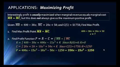
What is the antiderivative, and how is it used in the context of finding the exact total cost or revenue?
-The antiderivative is a function that reverses the process of differentiation. It is used to find the original function from its derivative. In the context of finding the exact total cost or revenue, one would find the antiderivative of the marginal cost or revenue function and evaluate it over the desired interval.
How does the concept of antiderivatives and areas apply to problem 38 in the transcript?
-In problem 38, the marginal cost function for producing jackets is given. To approximate the total cost of producing 400 jackets, one would calculate the total area under the curve of the marginal cost function using rectangles, which serves as an estimate since the actual function is not provided.
Outlines
📈 Introduction to Antiderivatives and Revenue Function
Professor Monty begins by introducing the concept of antiderivatives, explaining that they are a method of reversing the process of differentiation to find the original function from its derivative. Using the analogy of sales and revenue, he illustrates how knowing the rate of change (derivative) allows us to calculate the total revenue by finding the area under the derivative function's curve. This concept is fundamental to the section on antiderivatives as areas.
📊 Application of Antiderivatives in Cost Analysis
The professor moves on to an application of antiderivatives by examining a problem from the book. The problem involves finding the total cost of roasting coffee, given the marginal cost function. Without the original cost function, the professor demonstrates how to use the area under the marginal cost curve to estimate the total cost. This is done by plotting points and calculating the area under the curve, which represents the total cost.
🔍 Calculating Total Cost Using Marginal Cost
The video script details the process of calculating the total cost of producing a certain number of units using the marginal cost function. The professor uses a geometric approach to find the area under the curve of the marginal cost function by breaking it down into a rectangle and a triangle, then summing their areas to approximate the total cost. This method is a precursor to more advanced techniques that will be covered in later sections.
🔢 Approximating Area Under a Curve
The script discusses the process of approximating the area under a curve when the curve is not a straight line, such as a parabola represented by the function f(x) = x^2 + 1. The professor describes using rectangles to estimate the area under the curve, specifically by calculating the areas of three rectangles that fit under the curve and summing these areas for an approximation. This technique is a basic form of what will later be formalized using calculus.
📐 Geometry and the Limit of Rectangles
The professor explains that by increasing the number of rectangles used to approximate the area under a curve, the approximation becomes more accurate. The concept of taking the limit as the width of the rectangles approaches zero is introduced, which is a fundamental concept in calculus. The idea is that as the number of rectangles increases, their width decreases, leading to a better approximation of the actual area under the curve.
📉 Estimating Total Cost with Rectangles
The script presents a problem where the marginal cost for producing jackets is given, and the task is to approximate the total cost of producing 400 jackets. The professor outlines a method for using rectangles to estimate this total cost, noting that this approach will overestimate the actual cost due to the shape of the marginal cost curve. The process involves calculating the areas of four rectangles under the curve and multiplying by the common length to find the total estimated cost.
🧮 Antidifferentiation for Exact Total Cost
The final paragraph discusses the process of finding the exact total cost by antidifferentiating the marginal cost function. The professor indicates that by taking the antiderivative of the marginal cost function and evaluating it from the start to the end point, one can find the exact total cost. This approach is part of the next section's topic, which will delve deeper into the integral calculus required for these calculations.
Mindmap
Keywords
💡Antiderivatives
💡Derivative
💡Revenue Function
💡Marginal Cost
💡Total Cost
💡Graphing
💡Area Under the Curve
💡Linear Function
💡Trapezoid Rule
💡Approximation
💡Instantaneous Rate of Change
Highlights
Professor Monty introduces the concept of antiderivatives as a method to find the original function from its derivative, like finding the area under a rate of change curve.
The revenue function is exemplified by calculating total sales from a unit price and quantity, showcasing the relationship between price, quantity, and total revenue.
The graph of the derivative function (revenue per unit) is illustrated, emphasizing how the area under this graph correlates to the total revenue.
The idea that the area under the curve of the derivative equals the total change in the original function is established as a key principle.
An application problem from the book is introduced to demonstrate how to find the total cost from the marginal cost function without knowing the original cost function.
The process of finding the area under a linear marginal cost function using geometry is explained, highlighting the use of rectangles and trapezoids.
The concept of approximating the area under a curve by breaking it down into rectangles is introduced, with an example using a parabola.
The importance of using left-hand endpoints for approximating areas under a curve is discussed, noting the impact on the accuracy of the approximation.
An example calculation is provided to estimate the total cost of producing 400 jackets using the marginal cost function and the rectangle method.
The relationship between the number of rectangles used for approximation and the accuracy of the area under the curve is explored.
The idea of taking the limit as the width of the rectangles approaches zero to find the exact area under the curve is introduced.
An overview of how to find the exact total cost by antidifferentiating the marginal cost function is mentioned as a topic for a future section.
The method of approximating the area under a curve using rectangles is applied to a real-world problem involving cost analysis for jacket production.
The impact of the shape of the derivative function on the accuracy of the approximation is discussed, noting that non-linear functions require more rectangles for a good estimate.
The transcript concludes with a reminder of the upcoming section on calculus, which will cover finding exact areas under curves using integrals.
The importance of practicing the material and completing homework is emphasized to ensure a solid understanding of the concepts.
Transcripts

5.0 / 5 (0 votes)
Thanks for rating: