Avon High School - AP Calculus BC - Topic 10.12 - Example 2

Tony Record

7 Mar 202111:42

EducationalLearning

32 Likes 10 Comments

TLDRIn this engaging video, the presenter guides viewers through the process of using Taylor's inequality and the Lagrange error bound to approximate the value of e^x at x=1 with a third-degree polynomial. The step-by-step explanation involves calculating derivatives, evaluating them at zero for the Maclaurin polynomial, and then using the polynomial to estimate e. The video also demonstrates how to find the range of possible values for e^x at x=1 using the remainder term from Taylor's inequality, ultimately showing that the approximation falls within a range that closely matches the known value of e.

Takeaways

📘 The topic is the Lagrange Error Bound for approximating e^x at x=1 using a third-degree polynomial.
🌟 The process involves using Taylor's Inequality and not relying on memorization of the value of e.
🔍 The problem requires constructing the Taylor polynomial without it being explicitly given, starting from the original function e^x.
📈 The derivatives of e^x up to the third degree all evaluate to 1 at x=0, leading to a simple polynomial form.
🧮 The third-degree polynomial approximation for e^x at x=1 is 1 + (1/1!)x - 0^1 + (1/2!)x^2 - 0^2 + (1/3!)x^3.
🎯 The polynomial simplifies to 1 + x/2 + x^2/6, which when evaluated at x=1 gives 8/3 ≈ 2.67.
📊 Taylor's Inequality is used to find the range of possible values for e^x at x=1 by evaluating the remainder term.
🧬 The fourth derivative of e^x is e^x, which is constant and simplifies the process of finding the maximum value for the error bound.
🏹 A conservative estimate for the maximum value of the remainder term is used to ensure a safe error bound.
🤔 The final range of possible values for e^x at x=1, using the third-degree Maclaurin polynomial, is approximately between 2.61 and 2.73.
📚 The video emphasizes the importance of understanding the process and not just the final answer, and encourages further practice for better understanding.

Q & A

What topic is being discussed in the video?
-The topic being discussed is the Lagrange Error Bound and its application to find the third-degree polynomial approximation for e^x at x equals one, centered at zero.
Why is the topic of Lagrange Error Bound considered overwhelming for students?
-The topic is considered overwhelming because it involves understanding complex mathematical concepts, such as Taylor's inequality and polynomial approximations, which can be challenging for students who are new to these ideas.
What is the significance of the third-degree polynomial in this context?
-The third-degree polynomial is significant as it is used to approximate the function e^x at x equals one. This approximation helps in understanding the behavior of the function without relying on memorized values.
How many derivatives are taken to get to the third-degree polynomial?
-Three derivatives are taken to get to the third-degree polynomial, as it is a third-degree approximation.
What is the value of the third-degree polynomial at x equals one?
-The value of the third-degree polynomial at x equals one is 8/3, which is approximately 2.67.
What is Taylor's Inequality used for in this problem?
-Taylor's Inequality is used to find the range of possible values for e^x at x equals one by determining the maximum error that can occur using the third-degree polynomial approximation.
What is the role of the fourth derivative in the Lagrange Error Bound calculation?
-The fourth derivative plays a crucial role in the Lagrange Error Bound calculation as it represents the maximum value of the function's rate of change within the interval, which is used to estimate the error of the approximation.
How does the讲师 (instructor) handle the complexity of evaluating the fourth derivative at some point z between 0 and 1?
-The讲师 (instructor) chooses a conservative approach by evaluating the fourth derivative (which is e^x) at a point z slightly beyond 1 (using 3/4 as an example) to ensure a safe maximum value without needing a calculator.
What is the final range of possible values for e^x at x equals one, according to the video?
-The final range of possible values for e^x at x equals one, as determined using the Lagrange Error Bound, is between 2.67 (the approximation) and a value slightly greater than 2.718, which is close to the actual value of e.
How does the讲师 (instructor) encourage students to approach problems that seem overwhelming?
-The讲师 (instructor) encourages students to hang in there, to work through examples, and to check answers repeatedly. They emphasize that with practice, students will feel better about tackling complex topics.
What is the讲师's (instructor's) advice for dealing with the complexity of the Lagrange Error Bound?
-The讲师 (instructor) advises students not to let the complexity of the Lagrange Error Bound bother them. They suggest that sometimes, you just can't do anything about it and should focus on working through the problem without getting caught up in the details that might not be solvable without a calculator.

Outlines

00:00

📚 Introduction to Lagrange Error Bound

The video begins with an introduction to the concept of Lagrange Error Bound, emphasizing the importance of understanding the process rather than relying on memorization. The speaker encourages viewers to stick with the topic despite its complexity, assuring that familiarity will come with practice. The problem at hand involves finding a third-degree polynomial approximation for e^x at x=1, centered at zero, using Taylor's Inequality to determine the range of possible values for e^x at x=1. The speaker acknowledges the challenge but guides the audience through the steps of deriving the necessary polynomial and evaluating it at the given point.

05:02

🔢 Derivatives and Polynomial Construction

The speaker proceeds to calculate the derivatives of the exponential function e^x, which are all equal to e^x itself, and evaluates them at x=0 to construct the Maclaurin polynomial. The third-degree polynomial approximation is derived and simplified to 1 + (1/1!)x - (1/2!)x^2 + (1/3!)x^3. The video then moves on to approximate e^1 using this polynomial, resulting in a value close to the known approximate value of e. The speaker introduces Taylor's Inequality to find the range of possible values for e^x at x=1, explaining the concept of the remainder term and its calculation using the fourth derivative of the function.

10:04

📈 Lagrange Error Bound Application

The speaker applies the Lagrange Error Bound to determine the maximum possible error in the approximation of e^1. By evaluating the fourth derivative of e^x and finding its maximum value, the speaker calculates the bound of the error to be 1/8. The video then sets up an inequality to find the possible range of values for e^x at x=1, considering the error bound. The speaker solves this inequality to find the range of values that e^x at x=1 could fall within, which aligns with the known value of e. The video concludes with a reminder of the importance of understanding the process and the application of Taylor's Inequality and Lagrange Error Bound for error analysis in approximation problems.

Mindmap

Keywords

💡Lagrange Error Bound

The Lagrange Error Bound is a method used in calculus to estimate the error when approximating a function with a polynomial. In the context of the video, it is used to find the range of possible values for e^x at x=1 using a third-degree polynomial approximation centered at zero. The video explains how to apply this concept to determine the maximum possible error in the approximation, which is crucial for understanding the accuracy of the polynomial approximation.

💡Taylor's Inequality

Taylor's Inequality is a mathematical concept that provides an upper bound on the error when approximating a function with its Taylor series. In the video, Taylor's Inequality is used to find the range of possible values for e^x at x=1 by comparing the actual function value and the polynomial approximation. It is a key tool in the analysis of the accuracy of the approximation.

💡Maclaurin Polynomial

A Maclaurin Polynomial is a special case of the Taylor series where the expansion is centered at a point, typically zero. In the video, the Maclaurin Polynomial is constructed for the function e^x to approximate the value of e^1. The polynomial is derived by taking derivatives of the function and evaluating them at zero, which helps in understanding the approximation's accuracy.

💡Derivatives

Derivatives are a fundamental concept in calculus that represent the rate of change of a function. In the video, the speaker takes multiple derivatives of the function e^x to construct the Maclaurin Polynomial and to evaluate the Lagrange Error Bound. The derivatives of e^x are used to determine the coefficients of the polynomial and to find the maximum value of the error function.

💡Polynomial Approximation

Polynomial Approximation is the process of approximating a function with a polynomial expression. In the video, the speaker uses a third-degree polynomial to approximate the function e^x at x=1. This approximation is used to estimate the value of e^1 without relying on memorization and to understand the potential error in the approximation.

💡e to the power of x (e^x)

e^x is an exponential function where e is the base of the natural logarithm, approximately equal to 2.71828. In the video, the function e^x is the focus, and the speaker aims to approximate e^1 (e raised to the power of 1) using a polynomial. The value of e^1 is a well-known constant, and the video demonstrates how to find an approximation without relying on this prior knowledge.

💡Taylor Series

A Taylor Series is an infinite sum of terms that can be used to approximate functions. It is a representation of a function as the sum of its derivatives evaluated at a single point. In the video, the Taylor Series is used to approximate the function e^x with a polynomial centered at zero, which is a specific case known as a Maclaurin Series.

💡Approximation

Approximation in mathematics refers to the process of finding a value that is close to but not exactly equal to a given number or expression. In the video, the concept of approximation is central as the speaker uses a polynomial to approximate the value of e^1, providing an estimated value without using a calculator.

💡Error Analysis

Error Analysis is the process of estimating the magnitude of errors in a calculation or measurement. In the context of the video, Error Analysis is performed to determine the potential error in approximating e^1 using a third-degree polynomial. This is important for understanding the reliability of the approximation.

💡Factorial

A Factorial is a mathematical function that multiplies a given positive integer by all the positive integers less than it. It is denoted by the symbol '!' and is used in the video when constructing the Maclaurin Polynomial for e^x. Factorials appear in the coefficients of the polynomial terms.

💡Calculus

Calculus is a branch of mathematics that deals with rates of change and accumulation. In the video, calculus concepts such as derivatives, polynomial approximations, and Taylor series are used to analyze the function e^x and to perform error analysis. The video serves as an educational resource for understanding calculus applications.

Highlights

The topic is about using Taylor's Inequality to find the range of possible values for e^x at x=1 with a third-degree polynomial approximation centered at zero.

The process involves finding the third-degree polynomial approximation for e^x, which is an unusual problem as it essentially asks to determine e to the first power.

The Taylor polynomial is not given explicitly, so it must be constructed using derivatives of the function e^x.

The derivatives of e^x are all 1, making the construction of the Maclaurin polynomial straightforward.

The third-degree polynomial approximation is 1 + (1/1!)x - 0^1 + (1/2!)x^2 - 0^2 + (1/3!)x^3.

The polynomial simplifies to 1 + x/1! + x^2/2! + x^3/6, which approximates e^x at x=1 as 8/3 or 2.67, close to the actual value of e.

Taylor's Inequality is used to determine the range of possible values for e^x at x=1 by calculating the remainder term.

The remainder term is less than or equal to the absolute value of the maximum of the fourth derivative divided by 4! times (x-c)^(n+1), where z is between c and x.

The fourth derivative of e^x is simply e^x, which is constant and equal to 1 when evaluated at z.

A conservative approach is taken to estimate the maximum value of the remainder term by using a value of z slightly greater than 1.

The maximum bound of error is calculated to be 18/24 or 3/4, which is used to determine the possible range of values for e^x at x=1.

By solving the compound inequality, the possible range of values for e^x at x=1 is found to be between 23/24 and 41/24.

The actual value of e is approximately 2.71828, which falls within the calculated range using the third-degree Maclaurin polynomial.

The example demonstrates the practical application of Taylor's Inequality and the Lagrange error bound in approximating function values without a calculator.

The video is part of a series discussing Taylor's Inequality and its applications, with more examples and problems to be covered in class.

The use of Taylor's Inequality and the Lagrange error bound helps in understanding error analysis in approximations.

The video encourages viewers to practice and work through examples to build confidence in handling complex topics like Taylor's Inequality.

Transcripts

Browse More Related Video

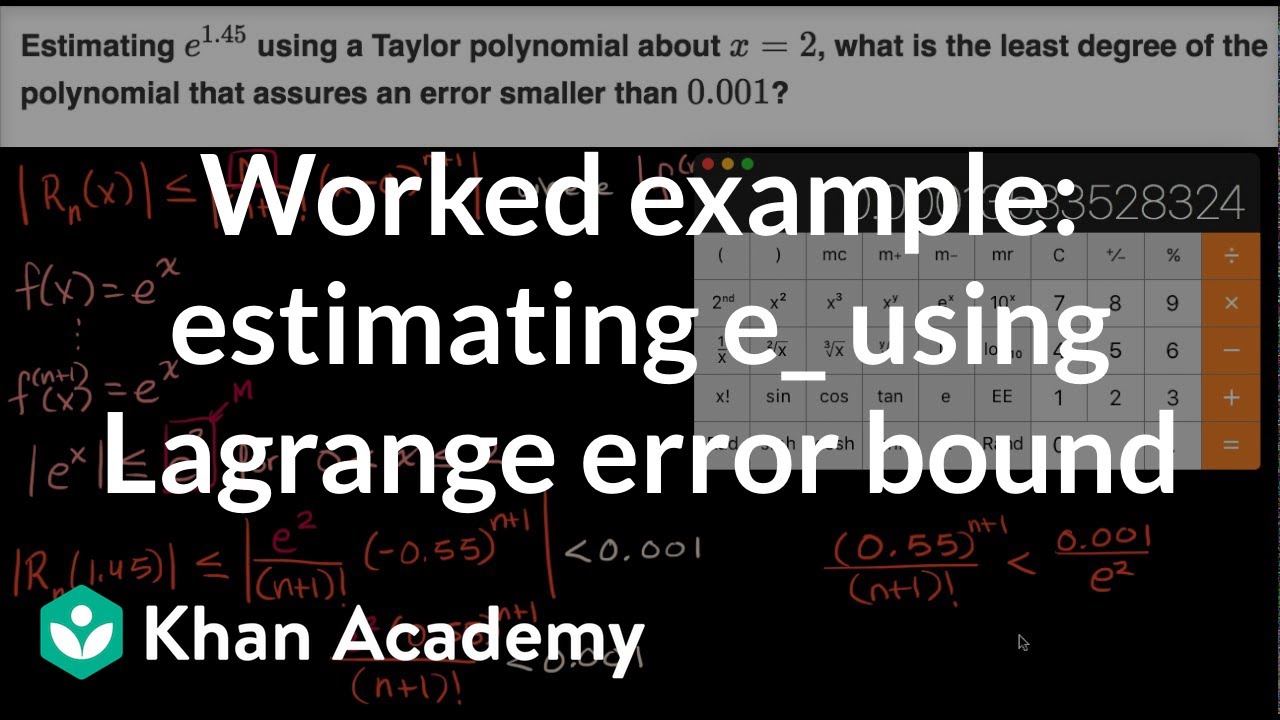
Worked example: estimating e_ using Lagrange error bound | AP Calculus BC | Khan Academy

2023 AP Calculus BC FRQ #6

Avon High School - AP Calculus BC - Topic 10.12 - Example 3

Worked example: Maclaurin polynomial | Series | AP Calculus BC | Khan Academy

Worked example: estimating sin(0.4) using Lagrange error bound | AP Calculus BC | Khan Academy

Worked example: Taylor polynomial of derivative function | AP Calculus BC | Khan Academy

Avon High School - AP Calculus BC - Topic 10.12 - Example 2

Takeaways

Q & A

What topic is being discussed in the video?

Why is the topic of Lagrange Error Bound considered overwhelming for students?

What is the significance of the third-degree polynomial in this context?

How many derivatives are taken to get to the third-degree polynomial?

What is the value of the third-degree polynomial at x equals one?

What is Taylor's Inequality used for in this problem?

What is the role of the fourth derivative in the Lagrange Error Bound calculation?

How does the讲师 (instructor) handle the complexity of evaluating the fourth derivative at some point z between 0 and 1?

What is the final range of possible values for e^x at x equals one, according to the video?

How does the讲师 (instructor) encourage students to approach problems that seem overwhelming?

What is the讲师's (instructor's) advice for dealing with the complexity of the Lagrange Error Bound?