9.1 Quantum Bound Eigenstates
TLDRThis lecture delves into the application of ordinary differential equations in quantum mechanics, specifically focusing on quantum bound states and eigenvalue problems. It explores the possibility of quantum mechanics within atomic nuclei, using computational tools to solve for energy levels of particles like neutrons and protons. The lecture introduces a numerical approach to match boundary conditions and solve the Schrödinger equation for various potentials, emphasizing the importance of accurate numerical methods like Runge-Kutta and the Numerov method. It concludes with an exercise for students to implement a bisection algorithm combined with an ODE solver to find precise energy levels, providing insights into the applicability of quantum mechanics in nuclear physics.
Takeaways
- 📚 The lecture is a supplementary session focusing on Chapter 9 of a textbook, which discusses ordinary differential equation applications in quantum mechanics.
- 🔬 The lecture explores two topics: quantum bound states and chaotic scattering, without introducing new algorithms but rather applying existing ones to solve eigenvalue problems.
- 🔍 A search algorithm is used in conjunction with an ordinary differential equation solver to tackle the eigenvalue problem, demonstrating the application of computational tools in physics.
- 🌌 The concept of quantum bound states is examined, including the possibility of quantum mechanics applying within atomic nuclei and the exploration of energy levels of particles like neutrons and protons.
- 📏 The size of an atomic nucleus is described, highlighting the vast difference in scale between the nucleus and the atom as a whole, and the challenge this presents in applying quantum mechanics.
- 🧬 The lecture delves into the quantum eigenvalue problem, explaining the physical assumptions made to simplify the problem to a time-independent Schrödinger equation.
- 🔑 The term 'bound state' is defined, emphasizing its physical meaning as a state confined to a specific region in space, and the mathematical approach to solving for it using eigenvalue problems.
- 📉 The importance of boundary conditions in solving differential equations is discussed, and how they are critical in determining the eigenvalues and eigenstates in quantum mechanics.
- 📈 The process of solving the bound state problem numerically is outlined, including the use of the Runge-Kutta method (RK4) and the Numerov method for solving the Schrödinger equation.
- 🔄 The technique of integrating the Schrödinger equation from both sides and matching the solutions at a 'matching radius' is explained to ensure the wave function and its derivative are continuous.
- 🔍 The use of a bisection algorithm to find the energy levels that satisfy the boundary conditions is suggested, emphasizing the precision and iterative nature of the computational approach.
Q & A
What is the main topic of the lecture?
-The main topic of the lecture is the application of ordinary differential equations in quantum mechanics, specifically in solving for quantum bound states and eigenvalue problems.
What are the two lectures mentioned in the script about?
-The two lectures mentioned are about quantum bound states and how to derive an eigenvalue problem from an ordinary differential equation, and chaotic scattering from a classical system.
Why does the lecturer emphasize the importance of using computational tools for new science and physics?
-The lecturer emphasizes the importance of computational tools because they allow researchers to solve complex problems, such as eigenvalue problems in quantum mechanics, which are beyond the scope of analytical solutions.
What is a quantum bound state in the context of this lecture?
-In the context of this lecture, a quantum bound state refers to a state in which a particle, like an electron or a nucleon, is confined to a specific region in space due to certain energy conditions.
What is the significance of the uncertainty principle in the context of electrons inside a nucleus?
-The uncertainty principle implies that if a very light particle like an electron is confined in a very small space, such as a nucleus, it would have an incredibly high momentum, which could lead to energetically unfavorable or unstable states.
Why is the time-independent Schrödinger equation used in this lecture?
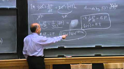
-The time-independent Schrödinger equation is used because it simplifies the problem by assuming that the time dependence of the wave function factors out, allowing researchers to focus on the spatial part of the wave function and its energy levels.
What is the physical interpretation of the term 'eigenvalue' in the context of quantum mechanics?
-In quantum mechanics, the term 'eigenvalue' refers to specific values, such as energy levels, that characterize the state of a quantum system. These eigenvalues are the solutions to the Schrödinger equation with specific boundary conditions.
What numerical methods are suggested for solving the Schrödinger equation in the script?
-The script suggests using the fourth-order Runge-Kutta method (RK4) or the Numerov method for solving the Schrödinger equation numerically.
How does the lecturer describe the process of solving the eigenvalue problem for quantum bound states?
-The lecturer describes the process as involving numerical integration of the Schrödinger equation from both sides of the potential well, matching the solutions at the boundary, and using a search algorithm to find the eigenvalues that satisfy the boundary conditions.
What is the role of the bisection algorithm in the context of this lecture?
-The bisection algorithm is used to find the eigenvalues of the quantum system by iteratively narrowing down the range of possible energies until the matching condition for the wave function is met within a specified tolerance.
How can one determine the ground state and excited states of a quantum system?
-One can determine the ground state and excited states by analyzing the wave functions and counting the number of nodes. The ground state has no nodes, while excited states have one or more nodes.
What is the significance of the potential well's depth in determining the existence of bound states?
-The depth of the potential well determines whether bound states exist. If the well is too shallow, there may be no bound states. As the well becomes deeper, it is more likely to support multiple bound states or eigenstates.
How does the mass of a particle affect the energy levels of a quantum system?
-The mass of a particle affects the energy levels because it influences the relationship between the wave vector and the energy. A lighter particle, like an electron, will have different energy levels compared to a heavier particle, like a nucleon, within the same potential well.
Outlines
📚 Introduction to Quantum Mechanics and Atomic Nucleus
The lecture begins by setting the stage for a supplementary discussion on ordinary differential equations, specifically focusing on quantum bound states and chaotic scattering. The speaker emphasizes the importance of using computational tools to explore physics, particularly quantum mechanics within the atomic nucleus. The historical context of 1920 is introduced to frame the question of whether quantum mechanics applies inside the nucleus. The lecture aims to illustrate the application of algorithms to new scientific problems, starting with the basics of atomic structure and the incredibly small scale of the nucleus compared to the atom as a whole.
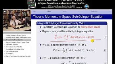
🔬 Quantum Bound States and the Schrödinger Equation
This section delves into the specifics of quantum bound states, explaining the physical concept as a state confined to a specific region in space. The mathematical formulation of this concept using the Schrödinger equation is discussed, with an emphasis on the eigenvalue problem that arises when seeking solutions where the wave function vanishes outside a certain region. The lecture introduces the idea of stationary states, simplifying the Schrödinger equation to a time-independent form, and discusses the significance of boundary conditions in defining these states.
📉 Mathematical Formulation of the Bound State Problem
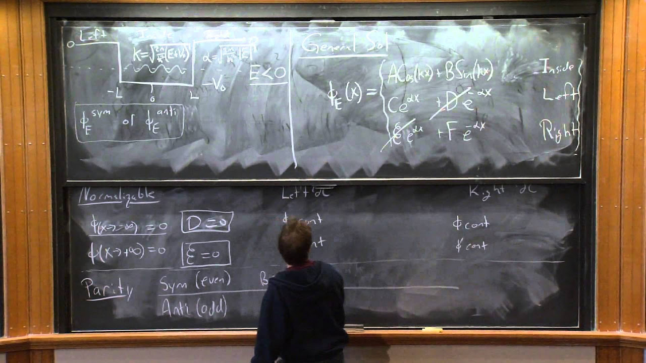
The script moves on to the mathematical formulation of the bound state problem, starting with the probability density function and its relation to the wave function. The time-independent Schrödinger equation is presented, highlighting the conditions for bound states, specifically that only negative energies can lead to bound states due to their decaying exponential solutions. The importance of the wave vector kappa and its relation to energy is explained, setting the stage for solving the second-order differential equation that describes the system.
🧬 Exploring the Quantum Eigenvalue Problem
The paragraph discusses the process of solving the quantum eigenvalue problem, which involves finding energies that satisfy both the differential equation and the boundary conditions. The concept of the ground state and excited states is introduced, with the ground state being the most negative energy solution. The importance of the wave function's curvature in relation to energy is highlighted, with the ground state having the least curvature. The paragraph also touches on the numerical methods for solving the Schrödinger equation, such as the Runge-Kutta method and the Numerov method.
🔧 Numerical Solution Techniques for the Schrödinger Equation
The focus shifts to the practical aspects of solving the Schrödinger equation numerically. The paragraph discusses the choice between using a simple finite square well potential for ease of explanation or more complex, realistic potentials. The numerical solution process involves integrating the differential equation both inside and outside the potential well and matching the solutions at the boundary. The importance of integrating inwards on growing functions to maintain accuracy is emphasized, and a technique for matching the solutions at the boundary is introduced.
🔄 Matching Solutions and the Bisection Algorithm
This section provides a detailed explanation of the technique for matching solutions obtained by integrating the Schrödinger equation from both sides of the potential well. The importance of the logarithmic derivative for ensuring the continuity of the wave function and its derivative is discussed. The paragraph introduces the use of a search algorithm, such as the bisection method, to find the energy values that result in a match between the left and right solutions. The need for precision in the numerical solution and the process of iterative refinement to achieve this precision is highlighted.
🔮 Conclusion and Practical Application
The final paragraph wraps up the lecture by summarizing the process and encouraging practical application of the concepts discussed. The speaker suggests using the bisection algorithm in conjunction with an ODE solver to find the energy levels of the system. The importance of verifying the solutions by checking the confinement of the wave function within the potential and counting the nodes to determine the state of excitation is emphasized. The lecture concludes with an invitation to experiment with different parameters, such as the mass of the particle, to explore the applicability of quantum mechanics to different physical systems.
Mindmap
Keywords
💡Ordinary Differential Equation (ODE)
💡Quantum Bound States
💡Eigenvalue Problem
💡Schrodinger Equation
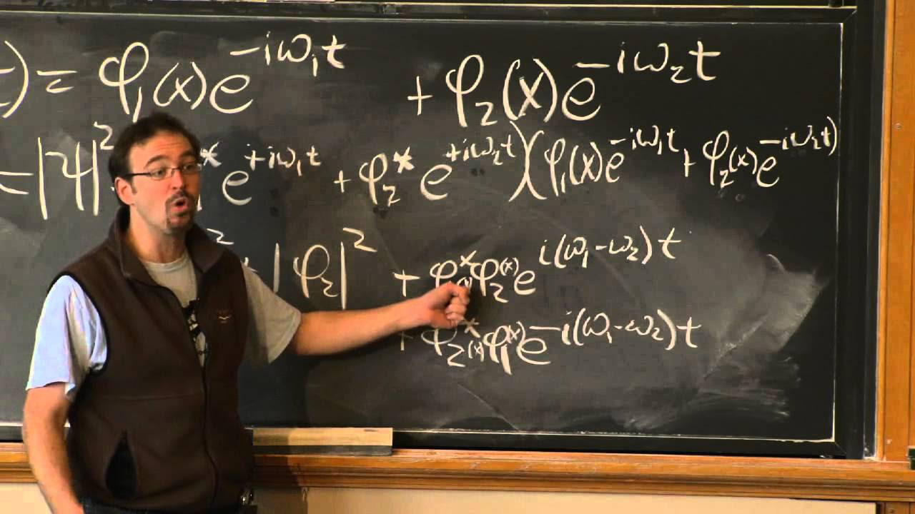
💡Stationary State
💡Boundary Conditions
💡Potential Well
💡Wave Function
💡Numerical Methods
💡Bisection Algorithm
💡Logarithmic Derivative
Highlights
Introduction to supplementary lectures on ordinary differential equation applications, specifically quantum bound states and chaotic scattering.
Discussion on the use of algorithms for solving eigenvalue problems in physics without introducing new algorithms.
Illustrative problem setup to explore if quantum mechanics applies inside an atomic nucleus, as a research question from the 1920s.
Explanation of the vast size difference between an atom and its nucleus, emphasizing the minuscule scale of the nucleus.
Assumption of stationary states to simplify the Schrödinger equation to an ordinary differential equation.
Definition and physical interpretation of bound states in quantum mechanics.
The eigenvalue problem formulation in quantum mechanics, linking it to the specific energy levels of bound states.
Numerical approach to solving the Schrödinger equation with the use of boundary conditions.
The importance of the wave function's modulus squared for calculating probability densities in quantum mechanics.
Assumption of negative energy for bound states leading to dying exponential solutions.
Description of the mathematical formulation for solving the bound state problem with a one-dimensional time-independent Schrödinger equation.
Use of wave vector kappa in the formulation of the Schrödinger equation for bound states.
Explanation of the process to solve the differential equation and impose boundary conditions for eigenvalue problems.
Choice between using RK4 or the Numerov method for solving ordinary differential equations in quantum mechanics.
Technique of integrating the Schrödinger equation from both sides and matching solutions at the potential boundary.
The importance of matching logarithmic derivatives for ensuring continuity in numerical solutions.
Use of a search algorithm to find the energy eigenvalue by minimizing the difference between logarithmic derivatives.
Exercise suggestion to implement the bisection algorithm combined with an ODE solver for finding energy levels.
Verification of the solution by ensuring the calculated energy levels are in the correct order of magnitude, such as millions of electron volts.
Final thoughts on the applicability of quantum mechanics to neutrons and protons within the nucleus and the historical significance of the problem.
Transcripts
Browse More Related Video

5.0 / 5 (0 votes)
Thanks for rating: