Lecture 11: Dispersion of the Gaussian and the Finite Well
TLDRThis lecture delves into the finite potential well problem in quantum mechanics, contrasting it with the infinite well and exploring its bound states. The professor guides through the mathematical formulation and boundary conditions, highlighting the discrete energy levels and the wave functions' behavior. By graphically solving the transcendental equation, insights into the energy eigenvalues and the impact of well depth and width on the number of bound states are provided. The lecture also touches on the delta function potential, revealing the unique bound state it supports, and sets the stage for further exploration of quantum mechanical systems.
Takeaways
- 📚 The lecture discusses the finite potential well, a theoretical model used to understand bound states in quantum mechanics.
- 🔍 The finite well is an idealized model with a piecewise constant potential, which is not realistic but very useful for study.
- 🧩 The potential well has a finite depth and width, creating conditions to explore energy eigenfunctions and eigenvalues.
- 🌐 The lecture introduces the concept of bound states as energy eigenstates that are exponentially localized and do not disperse over time.
- 📉 For bound states within a finite well, the wave function and its first derivative must be continuous everywhere, including at the boundaries of the well.
- 📈 The professor derives a transcendental equation relating the wave number (k) and the decay constant (alpha) to the energy levels of the well.
- 📊 A graphical method is used to solve the transcendental equation, plotting the tangent function against a circle to find intersection points representing energy levels.
- 🔑 The depth and width of the well affect the number of bound states, with deeper and wider wells supporting more states.
- 🔬 The lecture touches on the limit of an infinitely deep well, recovering the results for the infinite square well and its quantized energy levels.
- 🤔 The script raises questions about the behavior of wave functions and energy levels as the well becomes very shallow or very narrow, hinting at the approach to a delta function potential.
- 🔍 The delta function potential is discussed as a limit of a deep and narrow well, with the potential creating a kink in the wave function and supporting a single bound state.
Q & A
What is the main topic discussed in the lecture?
-The main topic discussed in the lecture is the finite potential well, also known as the finite well, and solving for its energy eigenfunctions and eigenvalues.
Why is the finite well model considered a useful toy model despite its unphysical discontinuity?
-The finite well model is considered useful because it allows for the study of bound states in quantum mechanics and can be used to approximate real-world systems like electric fields between capacitor plates, despite its piecewise constant and discontinuous nature.
What is the Schrodinger equation in the context of the finite well problem?
-The Schrodinger equation for the finite well problem is given by \( \phi''_e(x) = \frac{2m}{\hbar^2} (V(x) - E) \phi_e(x) \), where \( \phi_e(x) \) is the energy eigenfunction, \( E \) is the energy eigenvalue, \( V(x) \) is the potential function, \( m \) is the mass of the particle, and \( \hbar \) is the reduced Planck constant.
What are the boundary conditions for the finite well problem?
-The boundary conditions for the finite well problem are that the wave function and its derivative must be continuous at the boundaries of the well and that the wave function should vanish far away from the well to ensure normalizability.
How does the number of bound states in a finite well change as the well becomes deeper?
-As the well becomes deeper, the number of bound states increases because the larger potential well can support more energy levels below the potential barrier.
What is the significance of the transcendental equation derived for the finite well problem?
-The transcendental equation is significant because it provides a condition that relates the energy eigenvalues to the parameters of the well, such as its depth and width. Solving this equation yields the quantized energy levels of the bound states within the well.
How can the graphical solution method be used to solve the transcendental equation for the finite well?
-The graphical solution method involves plotting the functions representing the transcendental equation and finding their points of intersection, which correspond to the solutions of the equation. In the case of the finite well, one would plot the tangent function and circles representing the constant term, and the intersection points give the possible energy levels.
What is the physical interpretation of the wave function being continuous and having a continuous derivative at the boundaries?
-The physical interpretation is that the wave function and its first derivative must be smooth everywhere, which is a requirement for the system to have a well-defined energy eigenstate. This smoothness ensures that the particle's probability density and current are well-behaved at the boundaries of the potential well.
What happens to the ground state energy of the finite well as the well becomes wider?
-As the well becomes wider, the ground state energy decreases in magnitude, meaning the state becomes more deeply bound within the well due to the increased spatial extent available for the particle.
What is the relationship between the number of bound states and the depth of the potential well?
-The number of bound states is directly related to the depth of the potential well. A deeper well can support more bound states because it can accommodate more energy levels below the potential barrier.
Outlines
📚 Introduction to Finite Potential Well
The professor introduces the concept of a finite potential well, a theoretical model used in quantum mechanics to study bound states. Unlike real-world scenarios, this model assumes a potential that is piecewise constant, creating a simplified system to analyze. The lecture aims to solve for energy eigenfunctions and eigenvalues under specific boundary conditions, expecting discrete energies for bound states and continuous energies for scattering states.
🔍 Exploring Boundary Conditions and Wave Function Behavior
The discussion delves into the technicalities of boundary conditions for wave functions in regions of constant potential. The professor explains how to solve the energy eigenvalue equation in these regions and emphasizes the importance of continuity in wave functions and their derivatives at boundaries. The behavior of wave functions in the presence of potential steps and singularities, such as delta functions, is also explored, highlighting the resulting discontinuities in derivatives.
🌐 Understanding the Finite Well Potential and Bound States
The lecture continues with a detailed examination of the finite well potential, its parameters, and the quest to find bound states. The professor describes the mathematical approach to determine the wave function's behavior inside and outside the well, applying boundary conditions at infinity for normalizability and at the well's edges for continuity. The concept of bound states as energy eigenstates with exponential localization is introduced, contrasting with scattering states.
📉 Deriving the Wave Function for the Finite Well
Building upon the previous discussions, the professor focuses on the derivation of the wave function for the finite well, considering both symmetric and antisymmetric solutions. The mathematical formulation involves solving differential equations with boundary conditions that ensure the wave function and its derivative are continuous. The lecture also addresses the simplification that arises from the potential's symmetry, leading to either even or odd wave functions.
🔧 Solving for Energy Eigenvalues in the Finite Well
The professor outlines the process of finding discrete energy eigenvalues for the finite well potential by solving a transcendental equation derived from the boundary conditions. The challenge of solving this equation numerically is introduced, with suggestions to use software like Mathematica. A graphical method for understanding the solutions is also presented, involving the use of dimensionless variables and the concept of a circle in a plot.
📈 Graphical Solution and the Physics of Energy Eigenstates
The lecture presents a graphical method to solve the transcendental equation for energy eigenvalues, using a circle representation to find intersections with the tangent function. The graphical technique reveals insights into the energy eigenstates and their dependence on the well's depth and width. The professor discusses how the number of bound states changes with the well's depth and width, emphasizing that there is always at least one bound state in a 1D finite well potential.
🔬 Analyzing the Limiting Cases of the Finite Well
The professor explores the limiting cases of the finite well, such as the deep well limit that approximates an infinite well, and the behavior as the well becomes very shallow. The discussion includes the recovery of known results for the infinite square well and the implications of making the well wider or deeper on the energy eigenvalues. The analysis reinforces the understanding of bound states and their properties in the context of varying well parameters.
🤔 Considering the Delta Function Potential
Towards the end of the lecture, the professor raises the question of the delta function potential, which is a singular limit of the finite well. The discussion explores the implications of such a potential on the wave function, suggesting the presence of a kink due to the discontinuity in the first derivative of the wave function. The lecture concludes with the anticipation of addressing the delta function potential in more detail in subsequent classes.
🎓 Conclusion and Preview of Future Topics
In conclusion, the professor summarizes the key findings of the lecture, including the graphical solution for energy eigenvalues and the properties of bound states in a finite well. The lecture ends with a preview of the next topic, which involves the delta function potential and its implications for quantum mechanical systems, such as the binding of atoms.
Mindmap
Keywords
💡Bound States
💡Scattering
💡Finite Potential Well
💡Wave Functions
💡Energy Eigenstates
💡Schrödinger Equation
💡Boundary Conditions
💡Quantum Harmonic Oscillator
💡Delta Function Potential
💡Normalization
💡Transcendental Equation
Highlights
Introduction to the finite potential well and its significance as a model system for quantum mechanics.
Discussion on the piecewise constant potential and its application in modeling real-world systems like electric fields between capacitor plates.
Explanation of the Schrodinger equation and its role in finding energy eigenstates for time evolution studies.
Insight into the discrete nature of allowed energies in a finite well, contrasting with the continuous energy states above the potential.
Derivation of the equation for energy eigenvalue and its simplification for solving the finite well problem.
Boundary conditions for the finite well problem, emphasizing the continuity of the wave function and its derivative.
Solution strategies for energy eigenfunctions in regions of constant potential and the method of patching solutions at boundaries.
Analysis of the behavior of wave functions and their derivatives at continuous and discontinuous potentials.
Introduction to the concept of bound states and scattering states in quantum mechanics, with a classical analogy.
Definition and properties of bound states, including their exponential localization and time invariance.
Parameter definitions for the finite well potential and the approach to finding bound states with energy less than the potential.
Application of symmetry principles to simplify the solutions for energy eigenfunctions in a symmetric potential well.
Development of a transcendental equation for energy from the boundary conditions and its implications for the discreteness of energy levels.
Graphical method for solving transcendental equations and its application to determine the energy eigenvalues of the finite well.
Qualitative analysis of energy eigenvalues and the number of bound states as a function of well depth and width.
Limiting cases of the finite well problem, including the recovery of the infinite square well solution and the behavior of states at threshold.
Discussion on the appearance and disappearance of bound states and the characteristics of threshold states with long evanescent tails.
Investigation of the delta function potential as a limit of a deep and narrow well, and its effect on the wave function.
Conclusion on the existence of a single bound state for the delta function potential and the conditions for its appearance.
Transcripts
Browse More Related Video
Lecture 7: More on Energy Eigenstates
23. Quantum Mechanics V: Particle in a Box
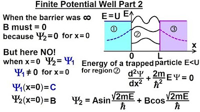
Physics - Ch 66 Ch 4 Quantum Mechanics: Schrodinger Eqn (33 of 92) Finite Potential Well Part 2

Quantum Physics: Part 2. Superposition. Particle in a box 🌚 Lecture for Sleep & Study
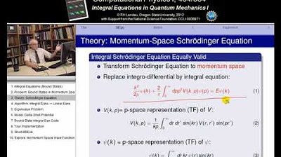
26.1 Integral Equations for Quantum Bound States
9.1 Quantum Bound Eigenstates
5.0 / 5 (0 votes)
Thanks for rating: