Warm up to the second partial derivative test
TLDRThis video script delves into the concept of finding maxima and minima in single and multi-variable calculus. It explains the process of setting the first derivative to zero for single-variable functions and the analogous method for multi-variable functions, which involves setting the gradient to the zero vector. The script also introduces the second derivative test for single-variable functions and hints at the second partial derivative test for multi-variable functions, which will be fully explained in a subsequent video. The example provided illustrates the process of finding where the gradient equals zero and sets the stage for a deeper exploration of the multi-variable second partial derivative test.
Takeaways
- 📚 In single variable calculus, to find the maximum or minimum of a function, you set its first derivative to zero, which corresponds to a flat tangent line on the graph.
- 🔍 The second derivative test in single variable calculus involves checking if the second derivative is greater or less than zero to determine if a point is a local maximum or minimum, respectively.
- 📈 The concept of concavity is used to understand the shape of the function's graph, with downward concavity indicating a local maximum and upward concavity indicating a local minimum.
- 🔬 In multi-variable calculus, finding local maxima or minima involves setting the gradient of the function to the zero vector, which corresponds to flat tangent planes.
- 🧩 The second partial derivative test is the multi-variable equivalent of the second derivative test in single variable calculus, used to determine the nature of critical points.
- 📝 The provided example function, f(x, y) = x^4 - 4x^2 + y^2, is used to illustrate the process of finding where the gradient equals zero.
- 🔑 The partial derivatives of the function with respect to x and y are set to zero to solve for critical points, resulting in three solutions: (0,0), (√2,0), and (-√2,0).
- 📊 The graph of the function helps visualize the nature of the critical points, showing that (0,0) is a saddle point and (√2,0) and (-√2,0) are local minima.
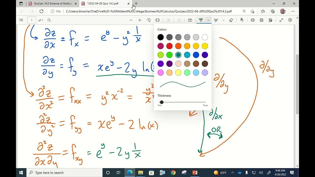
- 🔍 The second partial derivatives with respect to x and y are calculated to analyze the concavity in each direction, providing insight into the nature of the critical points.
- 🤔 The analysis of the second partial derivatives alone is not sufficient for a complete conclusion; the mixed partial derivative term must also be considered.
- 🚧 The video script concludes with a teaser for the next video, which will fully explain the second partial derivative test, including the mixed partial derivative term.
Q & A
What is the process to find the maximum or minimum of a single-variable function?
-To find the maximum or minimum of a single-variable function, you find its derivative and set it equal to zero. Graphically, this corresponds to finding points where the tangent line to the graph is flat.
How can you determine whether a critical point is a maximum, minimum, or neither by looking at the graph?
-By examining the concavity of the graph at the critical point. If the concavity is down, it's a local maximum; if it's up, it's a local minimum. If the concavity is flat, the second derivative test is inconclusive.
What is the second derivative test in the context of single-variable calculus?
-The second derivative test involves taking the second derivative of the function and checking its sign at the critical points. If the second derivative is less than zero, the point is a local maximum; if it's greater than zero, it's a local minimum.
How does the concept of finding maxima and minima differ in multi-variable calculus compared to single-variable calculus?
-In multi-variable calculus, you look for points where the gradient of the function is equal to the zero vector, indicating flat tangent planes instead of lines. This is analogous to setting the derivative equal to zero in single-variable calculus.
What is the second partial derivative test in multi-variable calculus?
-The second partial derivative test is used to determine the nature of critical points in multi-variable functions. It involves analyzing the concavity in multiple dimensions, including the mixed partial derivatives, to determine if a point is a local minimum, local maximum, or saddle point.
What is the significance of the mixed partial derivative term in the second partial derivative test?
-The mixed partial derivative term is crucial because it provides information about the concavity in different directions and helps to avoid incorrect conclusions about the nature of critical points, especially in cases where the analysis of individual variables might be misleading.
Can you provide an example of a multi-variable function and explain how to find where its gradient equals zero?
-The example given is f(x, y) = x^4 - 4x^2 + y^2. To find where the gradient equals zero, you set the partial derivatives with respect to x and y to zero and solve the resulting system of equations.
How do you interpret the solutions of the system of equations for partial derivatives in the context of the function f(x, y) = x^4 - 4x^2 + y^2?
-The solutions indicate the points (x, y) where the tangent plane to the function is flat. In the given example, the solutions are (0, 0), (sqrt(2), 0), and (-sqrt(2), 0), which correspond to potential local minima, maxima, or saddle points.
What does the second partial derivative with respect to x tell us about the concavity in the x direction?
-The second partial derivative with respect to x, 12x^2 - 8, indicates the concavity in the x direction at each point. A positive value suggests concavity up (local minimum), while a negative value suggests concavity down (local maximum).
How does the second partial derivative with respect to y help in understanding the concavity in the y direction?
-The second partial derivative with respect to y is simply 2, which is always positive. This indicates that there is always positive concavity in the y direction, suggesting that points could be local minima when considering only the y direction.
Why is it not sufficient to only consider the second partial derivatives with respect to individual variables?
-It is not sufficient because multi-variable functions can have complex concavity behaviors that are not captured by looking at individual variables alone. The mixed partial derivative term is necessary for a complete analysis.
Outlines
📚 Introduction to Maxima and Minima in Single and Multi-variable Calculus
This paragraph introduces the concept of finding maxima and minima in single-variable calculus by setting the first derivative to zero and using the second derivative test to determine if the point is a maximum or minimum. It then transitions into multi-variable calculus, where the gradient is set to the zero vector to find flat tangent planes. The analogy to the second derivative test in multi-variable calculus is introduced as the second partial derivative test, which will be explained in detail later in the video. A specific function, f(x, y) = x^4 - 4x^2 + y^2, is presented to demonstrate the process of finding where the gradient equals zero.
🔍 Solving for Critical Points and Analyzing Tangent Planes
The paragraph delves into solving the system of equations derived from setting the partial derivatives of the given function equal to zero. It explains how to find the critical points by solving for x and y, resulting in three solutions: (0,0), (√2,0), and (-√2,0). The speaker then discusses how to visually identify these points as saddle points or local minima by analyzing the graph. The concept of concavity in relation to the second partial derivatives is introduced to understand the nature of these critical points without relying on the graph.
🔄 The Importance of Mixed Partial Derivatives in Multi-variable Analysis
This paragraph emphasizes the limitations of analyzing concavity based solely on the second partial derivatives with respect to individual variables. It points out that mixed partial derivatives, which involve taking the derivative with respect to one variable and then with respect to another, are crucial for a complete analysis. The speaker mentions that a more comprehensive second partial derivative test, which includes the mixed partial derivative term, will be presented in the next video to avoid incorrect conclusions about the nature of critical points.
Mindmap
Keywords
💡Derivative
💡Flat Tangent Line
💡Second Derivative Test
💡Concavity
💡Gradient
💡Partial Derivative
💡Saddle Point
💡Second Partial Derivative Test
💡Mixed Partial Derivative
💡Function Extrema
💡Critical Points
Highlights
In single variable calculus, to find the maximum or minimum of a function, one sets its derivative equal to zero.
Graphically, setting the derivative to zero looks for points where the function has a flat tangent line.
A local maximum or minimum can be identified by the concavity of the function, determined by the second derivative.
In multi-variable calculus, the gradient of a function is set to the zero vector to find local extrema, analogous to setting the derivative to zero in single variable calculus.
The second partial derivative test is the multi-variable equivalent to the single variable second derivative test.
The function f(x, y) = x^4 - 4x^2 + y^2 is used as an example to demonstrate finding where the gradient equals zero.
Partial derivatives with respect to x and y are set to zero to find points of potential extrema.
Solving the system of equations from the partial derivatives yields three solutions: (0,0), (√2,0), and (-√2,0).
The point (0,0) is identified as a saddle point, neither a local maximum nor minimum, based on the graph.
The points (√2,0) and (-√2,0) are identified as local minima based on the graph's concavity.
The second partial derivative with respect to x is calculated to analyze concavity in the x-direction.
The second partial derivative with respect to y is constant and positive, indicating positive concavity in the y-direction.
The analysis of concavity in single directions (x and y) is not sufficient for full conclusions about extrema in multi-variable functions.
Mixed partial derivatives must be considered for a complete analysis of concavity and to avoid incorrect conclusions.
The video concludes with a promise to present the full second partial derivative test, including mixed partial derivatives, in the next installment.
Transcripts


5.0 / 5 (0 votes)
Thanks for rating: