Multivariable Optimization with Boundaries
TLDRThis video script delves into the process of finding global maximums and minimums of a multi-variable function within a closed and bounded region, contrasting it with finding local extrema. It revisits the concept of critical points and the second derivative test from single-variable calculus, then extends these methods to multi-variable functions. The script provides a step-by-step guide, including visualizing the function within a restricted domain, such as a cylinder, and finding the extrema on both the interior and the boundary of this domain. It introduces parameterization techniques to handle boundary curves and demonstrates how to apply calculus principles to find the absolute maximum and minimum values within a given domain, illustrating the application of the extreme value theorem.
Takeaways
- 📚 The video discusses finding global maximums and minimums of a multivariable function within a closed and bounded region, contrasting it with finding local extrema.
- 🔍 It reviews the method for finding local maximums and minimums by identifying critical points through setting partial derivatives equal to zero and using the second derivative test for classification.
- 📈 The script introduces a specific example function 2x^2 + y^2 - y with the constraint x^2 + y^2 <= 1, which visualizes as a parabola within a circular region.
- 📉 The video explains that the global minimum is visually identified within the circular region and can be found algebraically by setting partial derivatives to zero and solving for the variables.
- 🔑 The global maximum, however, is constrained to the boundary of the region, meaning it must occur on the circle defined by x^2 + y^2 = 1.
- 📐 The process of finding the maximum involves parameterizing the boundary using an angle θ and converting the multivariable function into a single-variable function of θ.
- 📝 By taking the derivative of the single-variable function and setting it to zero, the video shows how to find potential maximum and minimum points along the boundary.
- 📊 The script provides a step-by-step algebraic solution for the example, including finding critical points in the interior and on the boundary of the region.
- 🌐 The video mentions an alternative method of directly substituting the boundary condition into the original function to find extrema, instead of parameterization.
- 📚 The extreme value theorem is referenced, stating that a continuous function over a closed and bounded domain will attain a global maximum and minimum.
- 🔍 The takeaway is that to find the global extrema of a function within a closed and bounded region, one must check both the interior for critical points and the boundary for potential extrema.
Q & A
What are the different types of extrema that can be found in multivariable functions?
-In multivariable functions, there can be local minimums, where the point is smaller than everything around it, local maximums, and saddle points, which are interesting cases where in one direction it looks like it's increasing and in another direction it looks like it's decreasing.
What is the first step in finding local maximums and minimums of a multivariable function?
-The first step is to find the critical points of the function, which is where the partial derivative with respect to x and the partial derivative with respect to y are both equal to zero.
How is the second derivative test used to classify critical points in multivariable functions?
-The second derivative test involves analyzing second partial derivatives such as f_xx and f_xy. It provides information on whether a critical point is a local maximum, a local minimum, or a saddle point.
What does it mean to find extrema of a function on a closed region?
-Finding extrema on a closed region means that you are looking for the maximums and minimums of a function within a restricted area, such as inside a bounded domain or on the boundary of a region.
How does the closed bounded domain affect the process of finding extrema?
-The closed bounded domain imposes restrictions on where the extrema can occur. It means that you must consider points within the domain and on its boundary, potentially leading to global maximums or minimums that occur on the boundary.
What is an example of a closed bounded domain in the script?
-An example given in the script is the domain defined by x^2 + y^2 ≤ 1, which represents a circle with a radius of 1, including all points inside and on the boundary of the circle.
How does the intersection between a parabola and a cylinder visualize the problem of finding extrema on a closed region?
-The intersection between the parabola (2x^2 + y^2 - y) and the cylinder (x^2 + y^2 ≤ 1) visually represents the points where the function's values are considered, with the extrema potentially occurring either at the bottom of the parabola or along the boundary of the cylinder.
What is the extreme value theorem and how does it relate to finding global maximums and minimums?
-The extreme value theorem states that if a multivariable function is continuous on a closed and bounded domain, then it attains both a global maximum and a global minimum within that domain.
What are the two methods discussed in the script for finding extrema on the boundary of a region?
-The two methods discussed are parameterization of the boundary, using an angle theta to express the boundary curve in terms of a single variable, and direct substitution, where the boundary curve is substituted directly into the function to express it in terms of a single variable.
How does the parameterization method turn a multivariable function into a single variable function?
-By expressing the boundary curve in terms of a single parameter, such as theta for a circle (x = cos(theta), y = sin(theta)), the multivariable function can be rewritten as a function of that single parameter, allowing for the application of single-variable calculus techniques.
Outlines
📚 Introduction to Finding Extrema on a Closed Region
This paragraph introduces the concept of finding maximums and minimums of a multivariable function within a closed and bounded region. It contrasts this with the previous discussion on local extrema by explaining the impact of the closed region constraint. The speaker reviews the methods for identifying local minima, maxima, and saddle points, emphasizing the role of partial derivatives set to zero to find critical points. The second derivative test is mentioned as a means to classify these points. The paragraph sets the stage for a more complex scenario involving a parabola with a constraint, visualized as a cylinder, where the goal is to find the global extrema within this geometric constraint.
📈 Analyzing the Parabola and Cylinder Intersection
The speaker elaborates on the process of finding the global extrema of a function defined by 2x squared plus y squared minus y, subject to the constraint x squared plus y squared less than or equal to 1, visualized as a cylinder. The intersection of the parabola and the cylinder is highlighted, and the potential locations for global maxima and minima are discussed. The paragraph explains that without the cylinder constraint, the parabola would have no maximum, but with the constraint, the maximum occurs at specific points on the boundary curve. The speaker also mentions interesting points along the boundary that might be relevant to the analysis, setting up for an algebraic solution to find the exact extrema.
🔍 Algebraic Solution for Global Extrema
This paragraph delves into the algebraic method to determine the global extrema of the given function within the constrained region. The speaker first computes the critical point within the cylinder, finding it to be at (0, 1/2) with a function value of -1/4, which is claimed to be the local minimum. The second derivative test is applied to confirm this claim, using the condition that FXX is positive and the determinant of the Hessian matrix is also positive. The speaker then discusses the need to consider boundary points as potential extrema and introduces parameterization of the boundary using the angle theta, transforming the multivariable problem into a single-variable optimization problem. The derivative with respect to theta is computed, and the critical points along the boundary are determined by setting this derivative to zero.
📉 Evaluating Boundary Points and Applying the Extreme Value Theorem
The speaker continues the analysis by evaluating the boundary points identified through parameterization. A table is constructed to compare the function values at different theta values, which correspond to potential extrema along the boundary. The global maximum and minimum values are identified as 9/4 and -1/4, respectively. The speaker also touches upon alternative methods for incorporating the boundary into the function, such as direct substitution, and emphasizes the importance of the Extreme Value Theorem. This theorem states that if a function is continuous on a closed and bounded domain, it must attain a global maximum and minimum. The paragraph concludes by summarizing the two-step process of checking for extrema in the interior and on the boundary of the region.
Mindmap
Keywords
💡Multivariable Function
💡Local Maximums and Minimums
💡Saddle Point
💡Critical Points
💡Second Derivative Test
💡Closed and Bounded Domain
💡Global Maximum and Minimum
💡Boundary Points
💡Parameterization
💡Extreme Value Theorem
Highlights
Introduction to finding maximums and minimums of multivariable functions on a closed region.
Review of local maximums, minimums, and saddle points in multivariable functions.
Explanation of finding critical points using partial derivatives set to zero.
Use of the second derivative test to classify critical points.
Imposing restrictions on a multivariable function within a closed bounded domain.
Visualizing the problem with a parabola and a bounding cylinder.
Graphical identification of potential maximum and minimum points within the constrained region.
Algebraic computation to find the global minimum inside the cylinder.
Application of the second derivative test to confirm the local minimum.
Exploring boundary points as potential maximums or minimums.
Parameterization of the boundary curve using angle theta.
Transformation of a multivariable function into a single-variable function of theta.
Derivation and optimization of the function with respect to theta.
Solving for theta values that indicate potential maximum and minimum points on the boundary.
Comparison of boundary points with the graphical representation.
Identification of the global maximum and minimum values within the domain.
Discussion of alternative methods for incorporating the boundary curve into the function.
Introduction and application of the Extreme Value Theorem in multivariable calculus.
Summary of the process for finding maximums and minimums on both the interior and boundary of a region.
Transcripts
Browse More Related Video
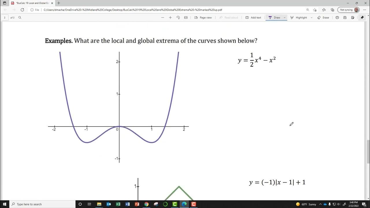
BusCalc 19 Local and Global Extrema
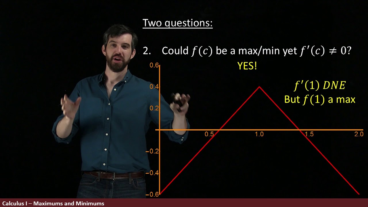
Relative and Absolute Maximums and Minimums | Part II

Calculus Review Maximum and Minimum Values of Functions

Lagrange Multipliers | Geometric Meaning & Full Example
Calculus 3: Maximum and Minimum Values (Video #17) | Math with Professor V
Calculus 1: Relative Extrema Examples
5.0 / 5 (0 votes)
Thanks for rating: