Second partial derivative test intuition
TLDRThis video script delves into the second partial derivative test, a method for determining local maxima, minima, or saddle points in functions of two variables. The process involves finding critical points where the gradient is zero and then calculating a value H using the second partial derivatives. If H is positive, the point is a local extremum; if negative, a saddle point. The script provides intuitive explanations for the test, including the significance of the mixed partial derivative and its role in capturing diagonal concavity disagreements.
Takeaways
- 📚 The second partial derivative test is used to identify local maxima, minima, or saddle points in multivariable functions.
- 🔍 The first step is to find critical points where the gradient equals zero, indicating all partial derivatives are zero.
- 🔢 The test involves computing the value H, which is the determinant of a matrix formed by second partial derivatives.
- 📉 If H > 0, the function has a local maximum or minimum, with the specific type determined by the sign of the second partial derivative in one direction.
- 📈 A positive second partial derivative in the x direction indicates a local minimum, while a negative indicates a local maximum.
- 📊 If H < 0, the point is a saddle point, indicating disagreement in concavity between different directions.
- ⚠️ If H = 0, the test is inconclusive, and further analysis is required to determine the nature of the critical point.
- 📐 The second partial derivative with respect to x (or y) treats the function as if x (or y) is the only variable, providing insight into concavity in that direction.
- 🔄 The mixed partial derivative captures the interaction between x and y directions, influencing the overall concavity of the function.
- 🤔 The test's effectiveness lies in its ability to assess concavity in all directions using just three second partial derivatives.
- 📘 For a rigorous justification of the second partial derivative test, an article with detailed explanations is available for interested viewers.
Q & A
What is the second partial derivative test used for?
-The second partial derivative test is used to determine whether a critical point of a two-variable function is a local maximum, local minimum, or a saddle point without having to visualize the graph.
What are critical points in the context of multivariable functions?
-Critical points are the points where the gradient of a multivariable function equals zero, indicating potential local maxima, minima, or saddle points.
What does the term 'H' in the second partial derivative test represent?
-The term 'H' represents the value obtained from the formula involving second partial derivatives, which is used to determine the nature of a critical point.
How does the value of 'H' indicate a local maximum or minimum?
-If the value of 'H' is greater than zero, it indicates that the critical point is either a local maximum or minimum, with the specific type determined by the sign of the second partial derivative in one direction.
What does a positive second partial derivative with respect to x indicate about the concavity in the x direction?
-A positive second partial derivative with respect to x indicates that there is positive concavity in the x direction, suggesting a local minimum.
What does a negative second partial derivative with respect to y indicate about the concavity in the y direction?
-A negative second partial derivative with respect to y indicates that there is negative concavity in the y direction, suggesting a local maximum.
What is a saddle point and how does the second partial derivative test identify it?
-A saddle point is a point which is neither a maximum nor a minimum. The test identifies it when the value of 'H' is less than zero, indicating disagreement in concavity in different directions.
What happens if the second partial derivatives with respect to x and y disagree in sign?
-If the second partial derivatives disagree in sign, it suggests a disagreement in concavity between the x and y directions, leading to a negative value of 'H' and identifying the point as a saddle point.
Why is the mixed partial derivative term important in the second partial derivative test?
-The mixed partial derivative term is important because it captures the disagreement in concavity along diagonal directions, which, when squared and subtracted, can influence whether 'H' is positive or negative.
What is the significance of the function f(x, y) = x * y in understanding the mixed partial derivative term?
-The function f(x, y) = x * y is significant because it graphically represents a saddle point, and its mixed partial derivative term equals 1, illustrating how the term captures diagonal disagreement in concavity.
If H equals zero, what does the second partial derivative test suggest?
-If H equals zero, the second partial derivative test is inconclusive, and additional methods are needed to determine the nature of the critical point.
Outlines
📚 Introduction to the Second Partial Derivative Test
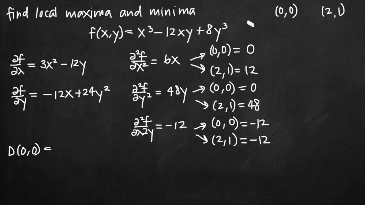
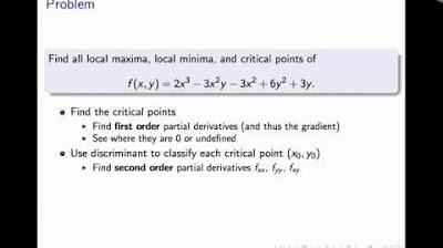
This paragraph introduces the second partial derivative test, a method used for multivariable functions, specifically two-variable functions, to identify local maxima, minima, and saddle points. The first step involves finding critical points where the gradient equals zero. The test then involves calculating the determinant of the Hessian matrix, which is a combination of the second partial derivatives with respect to x, the second partial derivatives with respect to y, and the mixed partial derivative. The sign of the determinant, H, indicates the nature of the critical point: positive indicates a local extremum, negative indicates a saddle point, and zero means the test is inconclusive. The paragraph also begins to explain the intuition behind the test, relating to the concavity in the x and y directions.
🔍 Understanding the Second Partial Derivative Test
This paragraph delves deeper into the second partial derivative test, explaining the significance of each term in the determinant H. It discusses how the second partial derivatives with respect to x and y indicate concavity in those directions, and how their product can indicate agreement or disagreement between the x and y concavities. The mixed partial derivative is highlighted as a term that captures diagonal disagreement in the function's behavior. The paragraph uses the function f(x, y) = x^2 - y^2 to illustrate a saddle point scenario and explains how the test works in such cases. It also mentions an article for those interested in a more rigorous justification of the test.
🤔 The Role of Mixed Partial Derivatives in the Test
The final paragraph focuses on the intuition behind the mixed partial derivative term in the second partial derivative test. It uses the simple function f(x, y) = xy to demonstrate how the mixed partial derivative can indicate disagreement in diagonal directions, which is key to identifying saddle points. The paragraph explains that even though there are infinitely many directions to consider, the mixed partial derivative, along with the pure second partial derivatives, is sufficient for the test. It suggests that the strength of the mixed partial derivative term can either pull the determinant H towards negativity, indicating a saddle point, or allow the agreement between x and y directions to dominate, indicating a local maximum or minimum. The paragraph concludes by referring to an article for a detailed explanation of the test.
Mindmap
Keywords
💡Second Partial Derivative Test
💡Multivariable Function
💡Critical Points
💡Gradient
💡Second Partial Derivatives
💡Mixed Partial Derivative
💡Local Maximum/Minimum
💡Saddle Point
💡Concavity
💡Diagonal Directions
Highlights
Introduction of the second partial derivative test for multivariable functions.
Finding critical points where the gradient equals zero in a two-variable function.
Explanation of the concept of concavity and its relation to local maxima and minima.
Computing the long value H using second partial derivatives to determine the nature of critical points.
Condition for H to indicate a local maximum or minimum: H must be greater than zero.
Determining concavity direction by examining the second partial derivative with respect to x or y.
Identification of a saddle point when H is strictly less than zero.
Inadequacy of the test when H equals zero, requiring additional methods for analysis.
Individual analysis of the second partial derivative with respect to x for x concavity.
Individual analysis of the second partial derivative with respect to y for y concavity.
The disagreement between x and y concavity leading to a saddle point.
Example function f(x, y) = x^2 - y^2 demonstrating disagreement in concavity.
Agreement between x and y directions for concavity and its effect on the value of H.
The role of the mixed partial derivative in capturing diagonal disagreement.
Graphical representation of the saddle point in the function f(x, y) = x * y.
Explanation of why only one mixed partial derivative is needed for diagonal direction analysis.
The battle between x and y agreement and the mixed partial derivative's influence on H.
Availability of a detailed article for those interested in the rigorous justification of the test.
Transcripts
Browse More Related Video

Second partial derivative test

Local Extrema, Critical Points, & Saddle Points of Multivariable Functions - Calculus 3

Second Derivative Test Multivariable (Calculus 3)
Local extrema and saddle points of a multivariable function (KristaKingMath)

BusCalc 14.3 Extrema of Multivariable Functions
Critical Points of Functions of Two Variables
5.0 / 5 (0 votes)
Thanks for rating: