Logistic Growth (Separable Differential Equations)
TLDRThe video script from Houston Math Prep discusses logistic growth, a type of exponential growth with a limit known as carrying capacity. The logistic growth equation is presented as DP/DT = R * (K - P)/K * P, where R is the growth rate, P is the current population, and K is the carrying capacity. The script breaks down the equation, showing how to solve it as a separable equation and eventually integrating it to find the population P as a function of time T. The process involves partial fraction decomposition and properties of logarithms and exponents. The final form of the logistic growth equation is derived, highlighting the interplay between the growth rate and the carrying capacity, and providing insight into how population growth is modeled under constraints.
Takeaways
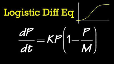
- 📈 **Logistic Growth Equation**: The population growth follows a logistic growth model, which is a type of exponential growth with a limit, expressed as DP/DT = R * (K - P)/K * P.
- 🔢 **Rate of Growth (R)**: 'R' in the equation represents the rate of growth, which can vary depending on the context.
- 🌱 **Current Population (P)**: 'P' is the current population at a given time, which influences the growth rate.
- 🚫 **Carrying Capacity (K)**: 'K' is the carrying capacity, a constant value that represents the maximum population size that the environment can sustain.
- 📉 **Growth Slowdown**: As the population approaches the carrying capacity, the growth rate slows down due to limited resources.
- 🧮 **Separable Equation**: The logistic growth equation is solved as a separable equation by isolating variables and integrating both sides.
- ✅ **Partial Fractions**: To integrate the equation, partial fractions are used to break down the complex fraction into simpler terms.
- 🔍 **Integration**: The integration process involves integrating with respect to 'P' and 'T', simplifying the equation to solve for 'P'.
- 🔁 **Logarithmic Properties**: Properties of logarithms are used to combine and simplify the integrated equation.
- 🌐 **Exponential Terms**: The solution involves exponential terms, showing how population growth is influenced by the rate 'R' and time 'T'.
- 🔗 **Final Form**: The final form of the logistic growth equation is P = K * C * e^(RT) / (1 + C * e^(RT)), where 'C' is a constant.
- ➗ **Dividing by Constant**: To normalize the equation, each term is divided by the constant 'C * e^(RT)', resulting in the common form of the logistic growth model.
Q & A
What is logistic growth?
-Logistic growth is a type of growth model that exhibits exponential growth at first but then slows down as it approaches a carrying capacity, which is a limit to how far the growth can go.
How is the logistic growth equation represented?
-The logistic growth equation is represented as DP/DT = R * (K - P)/K * P, where DP/DT is the change in population, R is the growth rate, P is the current population, and K is the carrying capacity.
What is the significance of the carrying capacity (K) in logistic growth?
-The carrying capacity (K) is the maximum population size that the environment can sustain indefinitely. It represents the limit to growth in logistic models.
What is the role of the growth rate (R) in logistic growth?
-The growth rate (R) is a constant that determines how quickly the population grows. It affects the initial exponential growth phase before the population begins to approach the carrying capacity.
How does the logistic growth model account for the slowing of growth as the population approaches the carrying capacity?
-The logistic growth model accounts for the slowing of growth through the term (K - P)/K, which represents the percent of carrying capacity left. As P approaches K, this term decreases, slowing the growth rate.
What is the method used to solve the logistic growth differential equation?
-The method used to solve the logistic growth differential equation is separation of variables, followed by integration with respect to P and T.
What is the purpose of separating variables in the logistic growth equation?
-Separating variables allows us to integrate each side of the equation with respect to its respective variable, which simplifies the process of finding the solution for P.
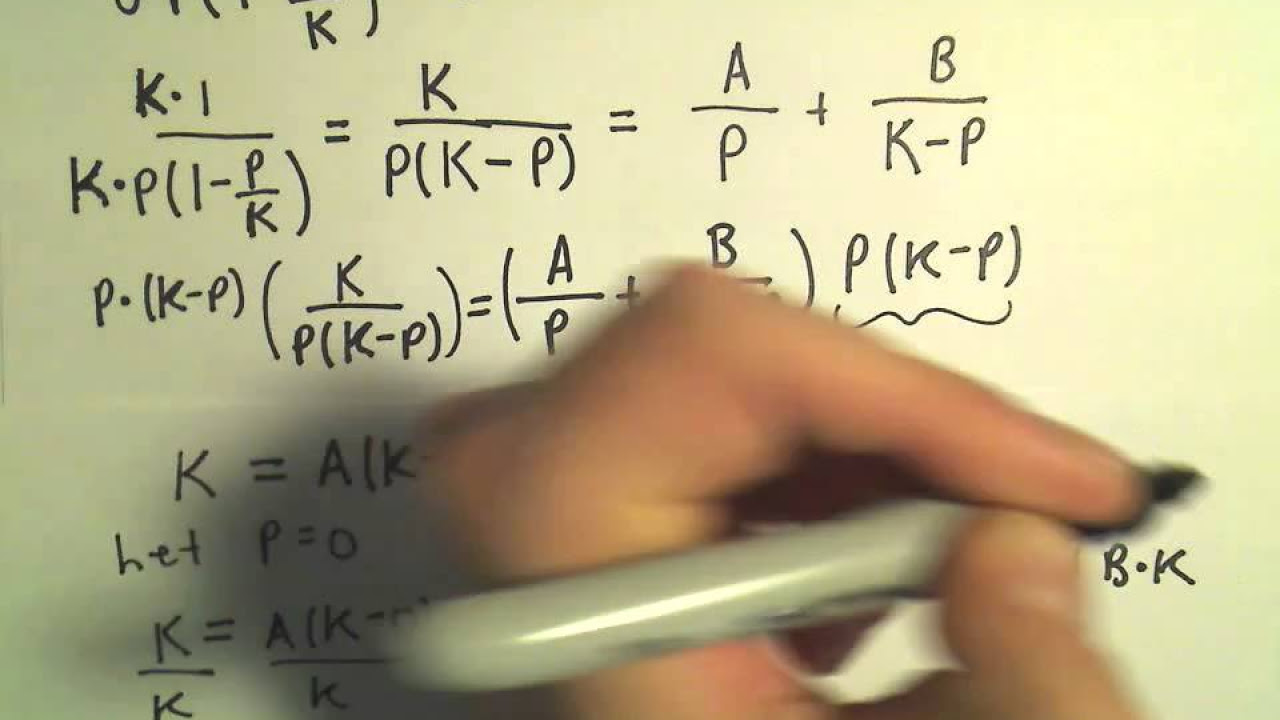
How are partial fractions used in solving the logistic growth equation?
-Partial fractions are used to break down the term K/(P * (K - P)) into simpler fractions that can be integrated more easily, facilitating the solution of the differential equation.
What is the final form of the logistic growth equation after solving for P?
-The final form of the logistic growth equation after solving for P is P = K * C * e^(RT) / (1 + C * e^(RT)), where C is a constant determined by initial conditions.
What does the term e^(RT) represent in the logistic growth equation?
-The term e^(RT) represents the exponential growth factor, where R is the growth rate and T is time. It accounts for the growth of the population over time.
How does the logistic growth model differ from the exponential growth model?
-The logistic growth model differs from the exponential growth model by incorporating a carrying capacity, which limits the growth of the population. This leads to a slowing of growth as the population size approaches the carrying capacity, unlike exponential growth which continues indefinitely.
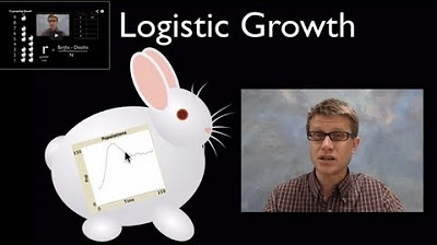
What are the practical applications of the logistic growth model?
-The logistic growth model is used in various fields to model population growth, such as in ecology to predict wildlife population dynamics, and in economics to forecast market growth, among other applications.
Outlines
📚 Introduction to Logistic Growth
The first paragraph introduces the concept of logistic growth, which is a form of exponential growth that includes a limiting factor, known as carrying capacity. This carrying capacity is the maximum population size that an environment can sustain indefinitely. The logistic growth equation is presented as DP/DT = R * (K - P) / K * P, where R is the growth rate, P is the current population size, and K is the carrying capacity. The paragraph explains each component of the equation and how the growth rate slows as the population approaches the carrying capacity.
🧮 Solving the Logistic Growth Differential Equation
The second paragraph delves into solving the logistic growth differential equation. It discusses the process of separating variables and integrating both sides of the equation with respect to P and T. The paragraph explains the use of partial fraction decomposition to simplify the integration process. It also covers solving for the constants a and B by substituting values for P that eliminate certain terms. The integration results in a natural logarithm relationship between P and T, which is then exponentiated to solve for P, leading to the logistic growth formula P = K * C * e^(RT) / (1 + C * e^(RT)), where C is a constant of integration.
🔍 Finalizing the Logistic Growth Equation
The third paragraph focuses on finalizing the logistic growth equation by making adjustments to the formula derived in the previous paragraph. It simplifies the equation by dividing each term by C * e^(RT), resulting in a more common form of the logistic growth model: P = K / (1 + (1/C) * e^(-RT)). The paragraph emphasizes that the rate R and the constant in the equation can influence the logistic growth pattern. It concludes by summarizing the insights gained from the logistic growth differential equation and the practice of separable equations.
Mindmap
Keywords
💡Logistic Growth
💡Exponential Growth
💡Carrying Capacity (K)
💡Rate of Growth (R)
💡Separable Equation
💡Partial Fractions
💡Integration
💡Differential Equation
💡Constant of Integration (C)
💡Limiting Value
💡Instantaneous Change
Highlights
Logistic growth is a type of exponential growth with a limit on how far the growth can go.
Population growth is influenced by the growth rate and the current size of the population.
The logistic growth model incorporates a carrying capacity, a maximum population size that cannot be exceeded.
The logistic growth equation is formulated as DP/DT = R * (K - P) * P / K, where R is the growth rate, P is the current population, and K is the carrying capacity.
The carrying capacity (K - P/K) represents the percentage of the carrying capacity that has not yet been reached.
The logistic growth equation is solved as a separable equation by isolating variables and integrating.
Partial fraction decomposition is used to simplify the integration process.
Integration involves finding antiderivatives with respect to both P and T.
The solution for P is obtained by applying properties of logarithms and exponents.
The final logistic growth model is presented as P/(K - P) = C * e^(RT), where C is a constant.
The constant C can be positive or negative, affecting the logistic growth curve.
The logistic growth model is applicable to both human populations and wildlife populations.
The model demonstrates how growth slows as the population approaches the carrying capacity.
The growth rate (R) remains a key factor in the logistic growth equation.
The model is solved by factoring out P and dividing by a term to isolate P.
The final form of the logistic growth equation is P = K * C * e^(RT) / (1 + C * e^(RT)).
The video provides a detailed walkthrough of solving the logistic growth differential equation.
The presenter emphasizes the importance of understanding separable equations in mathematical modeling.
The video concludes with a comprehensive understanding of how logistic growth models can be used in real-world scenarios.
Transcripts
Browse More Related Video

5.0 / 5 (0 votes)
Thanks for rating: