Average/Instantaneous Rates of Changes
TLDRThe video script provides an engaging introduction to the concepts of calculus, focusing on instantaneous and average rates of change. It begins with the fundamental functions of position (s(t)) and velocity (v(t)) over time, explaining their interrelation and importance in physics. The concept of average velocity is introduced through a practical example, emphasizing that it does not imply constant speed over time. The script then delves into the mathematical formula for calculating average velocity over a given time interval, using the position function s(t). The idea of instantaneous velocity is explored through the graphical representation of a position function, where the slope of the secant line connecting two points on the graph approximates the average velocity. The instantaneous velocity is defined as the limit of these secant lines as the time interval approaches zero, which is identified as the slope of the tangent line at a specific point. The video concludes with an example problem illustrating how to calculate instantaneous velocity using a position function, emphasizing the importance of approaching the point from both sides to ensure accuracy. This section of calculus serves as a foundation for further study in physics and introduces the concept of limits, which will be explored in more depth in subsequent sections.
Takeaways
- 📘 This video is a recap of Calculus 1 (Math 1321) at Baylor, based on Urgowski's fourth edition calculus textbook, focusing on section 2.1 about rates of change.
- 📐 Section 2.1 discusses two main types of rates: instantaneous and average rates of change, essential for understanding motion in physics.
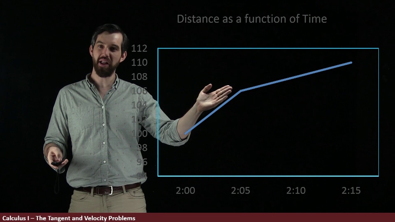
- 🏃 The video uses the example of running 200 miles in 4 hours to explain average velocity, highlighting that it doesn't reflect varying speeds throughout that period.
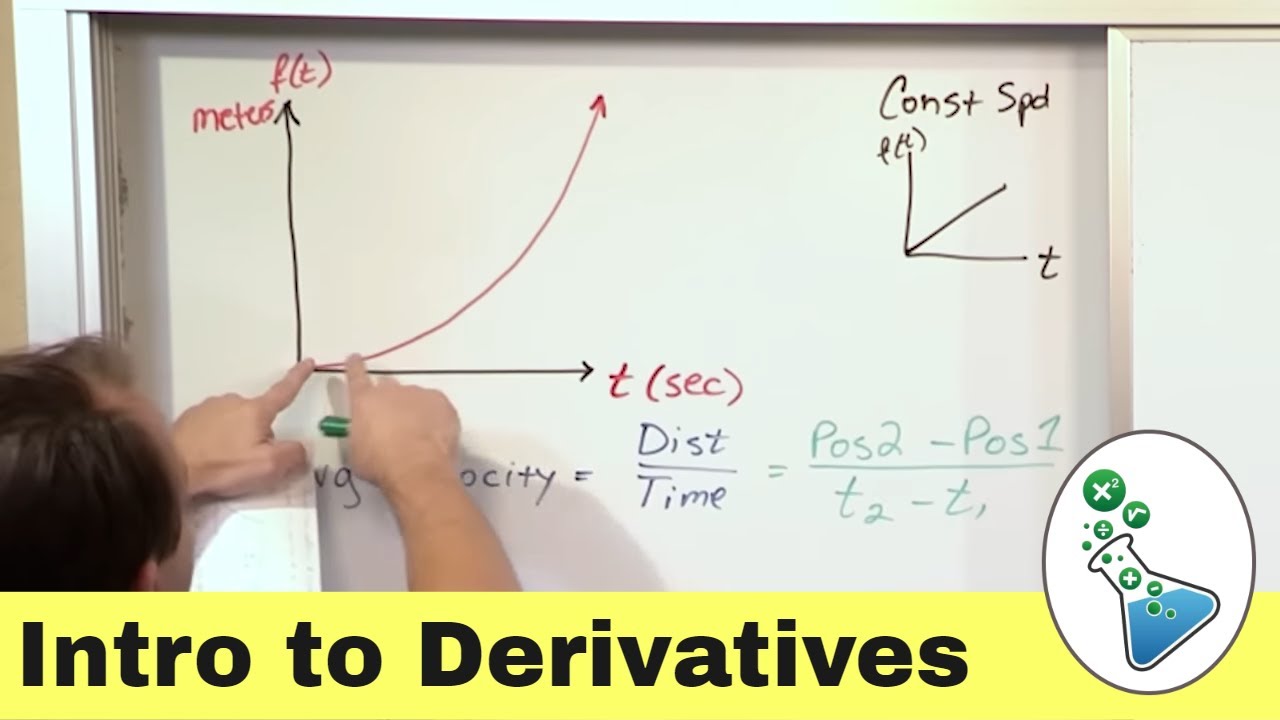
- 🔢 Two fundamental functions introduced are 's of t' for position and 'v of t' for velocity, emphasizing their critical relationship in calculus and physics.
- 🔍 Average velocity is calculated as the total change in position (delta s) divided by the total change in time (delta t).
- 📉 A practical formula for average velocity over a time interval uses the positions at the start and end of the interval divided by the time elapsed.
- 📚 A real-world example is used to apply the average velocity formula, where the position function is 't squared minus 2t plus 1'.
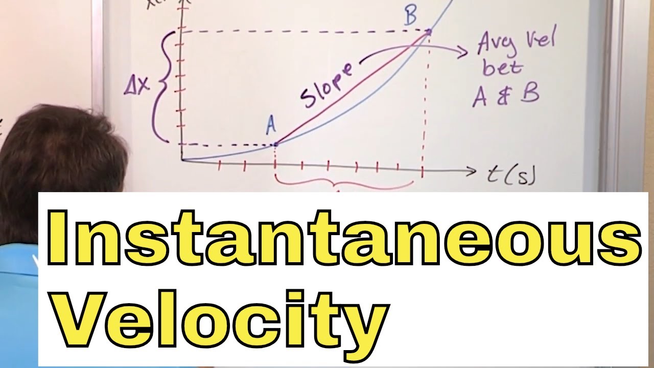
- 📈 The concept of the secant line is introduced as a geometric representation of average velocity, calculated from the slope of the line connecting two points on a graph.
- 🎯 Instantaneous velocity is defined as the limit of the average velocities as the time interval approaches zero, akin to the slope of the tangent line at a point.
- 🔄 The video demonstrates the process of finding instantaneous velocity through a detailed example involving limits, showing calculations from both sides of a specific point to ensure accuracy.
Q & A
What is the main focus of Section 2.1 in the calculus textbook?
-Section 2.1 focuses on instantaneous rates of change and the average rate of change, which are used to define the instantaneous rate of change.
What do the variables s(t) and v(t) typically represent in calculus?
-In calculus, s(t) typically stands for position at time t, and v(t) stands for velocity at time t.
Why was calculus largely developed?
-Calculus was largely developed to help prove physics, which is why we're interested in both position and velocity.
What does delta (Δ) represent in the context of the script?
-In the context of the script, delta (Δ) represents a change in a quantity, so Δs stands for change in position and Δt stands for change in time.
How is average velocity calculated?
-Average velocity is calculated as the total change in position divided by the total change in time.
What is the formula for average velocity given a time interval from t0 to t1 and a position function s(t)?
-The formula for average velocity is s(t1) - s(t0) divided by (t1 - t0), where s(t1) is the terminal position, s(t0) is the initial position, and t1 and t0 are the times.
What is the term for the line that connects two points on a graph, representing the average velocity over an interval?
-The term for the line that connects two points on a graph is a secant line.
How is instantaneous velocity defined?
-Instantaneous velocity is defined as the slope of the tangent line to the graph of a position function at a specific point, which is found by taking the limit of the average velocities as the time interval shrinks to zero.
What is the instantaneous velocity formula at a point t0?
-The instantaneous velocity formula at a point t0 is the limit as t1 approaches t0 of (s(t1) - s(t0)) / (t1 - t0).
Why is it important to approach a point from both sides when calculating instantaneous velocity?
-Approaching a point from both sides helps to ensure that the calculated instantaneous velocity is accurate and that the limit exists, providing a more robust verification of the result.
What is the significance of limits in calculus, as hinted in the script?
-The significance of limits in calculus is to study what happens as we approach certain values, which is foundational for understanding concepts like instantaneous velocity and is a topic that will be explored in more depth in subsequent sections.
Outlines
📚 Introduction to Calculus Concepts
The first paragraph introduces the topic of calculus, specifically focusing on instantaneous and average rates of change. The script uses the context of a calculus class at Baylor University and references the textbook by Urgowski. It explains the relevance of calculus to physics, particularly in relation to position and velocity. The concept of average velocity is introduced through an example of running 200 miles in four hours, leading to the formula for average velocity as change in position over change in time. The paragraph also outlines how to calculate average velocity given a time interval and a position function.
🏃♂️ Average and Instantaneous Velocity
The second paragraph delves deeper into the concept of velocity, differentiating between average and instantaneous velocity. It uses the example of a cheetah running 200 miles in four hours to illustrate the concept. The script explains how to represent this scenario with a position function and how to calculate the average velocity over a given time interval. It then transitions to the idea of instantaneous velocity, which is determined by the slope of the tangent line to a graph at a specific point. The paragraph also discusses the graphical representation of average velocity as the slope of a secant line between two points on a graph.
🚀 Calculating Instantaneous Velocity
The third paragraph focuses on the mathematical process of finding the instantaneous velocity at a specific point in time. It explains the concept of limits and how they are used to determine the instantaneous velocity by shrinking the time interval around the point of interest. The script provides a detailed example using a position function s(t) = t^3 - 3t and an initial time of t not equals 2. It demonstrates the process of taking the limit of average velocities as the time interval approaches zero, resulting in the instantaneous velocity at that point.
🔍 Limits and Approaching Values
The fourth and final paragraph reinforces the concept of limits in calculus and its importance in deriving instantaneous velocity from average velocity. It suggests verifying the calculated instantaneous velocity by approaching the point of interest from both directions, thereby ensuring the value is consistent. The paragraph concludes by highlighting the foundational role of calculus in physics and teases the upcoming discussion on limits in more depth in the following chapter. It summarizes the key topics covered in section 2.1, which include average velocity over a time interval and instantaneous velocity at a specific time.
Mindmap
Keywords
💡Instantaneous Rate of Change
💡Average Rate of Change
💡Position Function (s(t))
💡Velocity Function (v(t))
💡Delta (Δ)
💡Secant Line
💡Tangent Line
💡Limit
💡Slope
💡Time Interval
💡Integration with Physics
Highlights
Introduction to instantaneous and average rates of change as fundamental concepts in calculus.
The relationship between position (s(t)) and velocity (v(t)) functions and their significance in physics.
Explanation of delta s and delta t representing changes in position and time, respectively.
Calculation of average velocity as the total change in position divided by the total change in time.
Illustration of the concept of average velocity using an example of running 200 miles in four hours.
Differentiation between average velocity and instantaneous velocity, emphasizing the need for the latter to understand speed at a specific instant.
Use of a position function to represent an object's movement over time and how to calculate the average velocity for a given time interval.
Graphical representation of position functions and the concept of secant lines to approximate average velocity.
Introduction to the tangent line as a representation of instantaneous velocity at a specific point on a graph.
Demonstration of how to calculate the instantaneous velocity using the limit of average velocities as the time interval approaches zero.
Working example to find the instantaneous velocity at a specific time using the position function s(t) = t^3 - 3t.
Technique of using a table to list intervals and calculate the average velocity to find the limit for instantaneous velocity.
Approach to finding instantaneous velocity from both sides (approaching from values greater and lesser than the specific instant) to ensure accuracy.
The importance of limits in calculus as a method to understand instantaneous velocity and other derived quantities from average rates.
Connection between calculus and physics, emphasizing the foundational role of calculus in understanding physical phenomena.
Teasing the upcoming topic of limits in chapter 2, which will be explored in more depth.
Summary of the main topics covered in section 2.1, including average and instantaneous velocity calculations.
Practical application of these concepts in understanding an object's speed at a specific moment in time.
Transcripts
Browse More Related Video
Intro to Derivatives, Limits & Tangent Lines in Calculus | Step-by-Step
The Velocity Problem | Part II: Graphically
07 - What is Instantaneous Velocity?, Part 1 (Instantaneous Velocity Formula & Definition)

College Physics 1: Lecture 7 - Instantaneous Velocity

Two-Dimensional Motion and Velocity | Physics with Professor Matt Anderson | M4-02
Business Calculus - Math 1329 - Section 2.1 - The Derivative
5.0 / 5 (0 votes)
Thanks for rating: