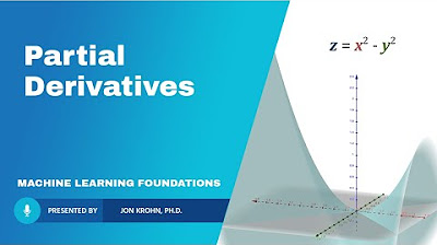
Partial Derivatives
TLDRThe video script provides an insightful discussion on partial derivatives, a concept from multivariable calculus. It reassures viewers that calculating a partial derivative is not more difficult than calculating a normal derivative and uses the same tools. The script explains that a partial derivative measures how a function changes when varying only one of its variables, keeping others constant. It uses the example of a function \( f(X, Y, Z) = 2Y^2 + X^2 \cos(Z) \) to demonstrate how to calculate the partial derivatives with respect to \( X \), \( Y \), and \( Z \). The video also touches on higher-order derivatives and mixed second derivatives, encouraging viewers to try these calculations as an exercise. The presenter emphasizes the ease of taking partial derivatives by treating all other variables as constants, just like in regular derivatives.
Takeaways
- 📚 Partial derivatives are part of multivariable calculus and can seem intimidating, but they are not more difficult than normal derivatives.
- 🔑 A partial derivative tells you how a function of multiple variables changes as you vary only one of its arguments, keeping others constant.
- 📈 The concept is similar to normal derivatives; it informs about the rate of change of a function with respect to one variable.
- 📝 Partial derivatives are denoted using a curly '∂' instead of the regular 'd' to differentiate from total derivatives.
- 📐 The partial derivative of a function with respect to a variable is found by differentiating that function with respect to the variable, treating all other variables as constants.
- 🌟 The rules for differentiation, such as the power rule, apply to partial derivatives in the same way as they do to regular derivatives.
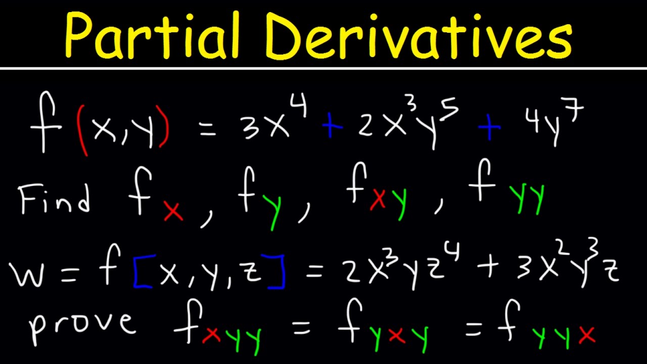
- 📙 Example provided in the script: For a function f(X, Y, Z) = 2Y^2 + X^2 * cos(Z), the partial derivatives with respect to X, Y, and Z are calculated by treating the other variables as constants.
- 🔍 The partial derivative with respect to X of the example function is 2Y^2 + 2X * cos(Z), treating Y and Z as constants.
- 🔎 The partial derivative with respect to Y of the example function is 4Y, with X and Z treated as constants, and the term not involving Y becomes a constant with a derivative of 0.
- 🧮 For the example function, the partial derivative with respect to Z is X^2 * sin(Z), since X and Y are treated as constants and the derivative of cos(Z) is -sin(Z).
- 🎓 Higher-order partial derivatives can also be taken, such as second or third order derivatives, which are an extension of first-order partial derivatives.
- 🤔 Mixed second derivatives can be calculated by taking the partial derivative with respect to one variable and then with respect to another, treating the first variable as constant in the second step.
Q & A
What is a partial derivative?
-A partial derivative tells you how a multivariable function changes as you vary only one of its arguments while keeping all other variables constant.
Why is multivariable calculus considered more complex than single-variable calculus?
-Multivariable calculus is considered more complex because it deals with functions that depend on more than one variable, requiring the use of partial derivatives to understand how the function changes with respect to each variable individually.
How is taking a partial derivative similar to taking a normal derivative?
-Taking a partial derivative is similar to taking a normal derivative in that the same rules and techniques apply. The main difference is that in a partial derivative, all other variables are treated as constants.
What does the symbol ∂ represent in mathematics?
-The symbol ∂ represents a partial derivative in mathematics, distinguishing it from a total or ordinary derivative.
What does the term 'f with respect to X' mean?
-The term 'f with respect to X' means the derivative of the function f taken with respect to the variable X, considering all other variables as constants.
How does the position of a particle relate to derivatives?
-The position of a particle can be described by a function of time. Taking the derivative of this function with respect to time gives the velocity of the particle, showing how the position changes over time.
Can you provide an example of a multivariable function?
-An example of a multivariable function is f(X, Y, Z) = 2Y^2 + X^2 * cos(Z), which depends on three variables X, Y, and Z.
What is the partial derivative of f with respect to X for the given example function?
-The partial derivative of f with respect to X for the function f(X, Y, Z) = 2Y^2 + X^2 * cos(Z) is ∂f/∂X = 2Y^2 + 2X * cos(Z).
How does the process of taking a partial derivative with respect to Y differ from taking it with respect to X?
-When taking a partial derivative with respect to Y, you treat X and Z as constants and differentiate the function only with respect to Y. In contrast, when taking it with respect to X, Y and Z are treated as constants.
What is the partial derivative of the example function with respect to Z?
-The partial derivative of the function f(X, Y, Z) = 2Y^2 + X^2 * cos(Z) with respect to Z is ∂f/∂Z = -X^2 * sin(Z).
Can higher-order partial derivatives be taken, and what are they?
-Yes, higher-order partial derivatives can be taken. They are derivatives of the first-order partial derivatives. For example, taking the second derivative of f with respect to X would involve differentiating the first-order partial derivative with respect to X again.
What is a mixed second derivative, and how is it different from a regular second derivative?
-A mixed second derivative is a second derivative where you first take the partial derivative with respect to one variable and then with respect to another. It differs from a regular second derivative in that the order of differentiation with respect to different variables is considered.
Outlines
📚 Introduction to Partial Derivatives
This paragraph introduces the concept of partial derivatives as a fundamental part of multivariable calculus. The speaker reassures the audience that despite the intimidating name, taking a partial derivative is not more difficult than taking a regular derivative. The tools used for regular derivatives apply to partial derivatives as well. The paragraph explains that a partial derivative describes how a function of multiple variables changes when only one variable is varied, while the others are held constant. The mathematical notation for partial derivatives is introduced, using a curly 'D' or 'f_x' to denote the derivative of 'f' with respect to 'X'. The explanation is supplemented with an example function involving variables X, Y, and Z, and the process of finding the partial derivative with respect to X is worked through step by step, treating Y and Z as constants.
🔍 Deriving Partial Derivatives and Their Applications
The second paragraph continues the discussion on partial derivatives by illustrating how to find the partial derivative of the same function with respect to Y and Z. It emphasizes that the process is as straightforward as taking normal derivatives, applying the same mathematical rules such as the power rule. The partial derivative with respect to Y is calculated, treating X and Z as constants, and the derivative of Y squared is identified. For the partial derivative with respect to Z, the process is shown to involve recognizing Z as the only variable in the term and differentiating it while treating X and Y as constants. The paragraph concludes with an encouragement to practice taking higher-order derivatives, such as second or third order, and to explore mixed second derivatives, which involve taking partial derivatives in a sequence of different variables. The speaker offers to answer any questions and thanks the audience for watching.
Mindmap
Keywords
💡Partial Derivatives
💡Multivariable Calculus
💡Derivative
💡Variables
💡Constant
💡Function
💡Higher-Order Derivatives
💡Mixed Second Derivatives
💡Power Rule
💡Cosine Function
💡Sine Function
Highlights
Partial derivatives are part of multivariable calculus and are used to determine how a function changes when varying only one of its arguments.
Taking a partial derivative is no more difficult than taking a normal derivative, using the same tools and rules.
A partial derivative tells you how a multivariable function's position changes when adjusting only one variable, similar to velocity in the context of changing time.
The notation for a partial derivative uses a curly D to differentiate it from a full derivative.
The partial derivative of a function F with respect to one variable X is written as ∂F/∂X or f_x, indicating the derivative of F with respect to X while treating all other variables as constants.
The process of taking a partial derivative involves differentiating the function with respect to one variable while considering the others as constants.
An example function f(X, Y, Z) = 2Y^2 + X^2 * cos(Z) is used to demonstrate the process of taking partial derivatives.
The partial derivative of the example function with respect to X is 2Y^2 + 2X * cos(Z), showing that constants come along for the ride and variables are treated as changing.
For the example function, the partial derivative with respect to Y is 2X * cos(Z), as Y^2 is treated as a constant and the derivative of a constant is zero.
The partial derivative with respect to Z of the example function is X^2 * sin(Z), as X and Y are treated as constants and the derivative of cos(Z) is -sin(Z).
Higher-order partial derivatives can also be taken, such as second or third order derivatives, which are an extension of first-order derivatives.
Mixed second derivatives can be calculated by taking the partial derivative with respect to one variable and then with respect to another, treating the previously derived variable as a constant.
The video challenges viewers to take the second derivative of the example function with respect to X as an exercise.
The presenter emphasizes that taking partial derivatives follows the same rules as taking normal derivatives, making the process straightforward once the concept of treating other variables as constants is understood.
The video concludes by encouraging viewers to ask questions if they have any, indicating an open invitation for further discussion and clarification.
Transcripts
Browse More Related Video


5.0 / 5 (0 votes)
Thanks for rating: