Partial derivatives, introduction
TLDRThis video script delves into the concept of partial derivatives for multi-variable functions, drawing parallels with ordinary derivatives. It explains the process of calculating partial derivatives by treating one variable as constant while differentiating with respect to the other. The script uses the function F(X, Y) = X^2 * Y + sin(Y) as an example to illustrate the computation of partial derivatives both at a specific point and as a general formula. It emphasizes the importance of understanding derivatives beyond the graphical representation, especially in higher dimensions, by focusing on the ratio of output change to input change.
Takeaways
- 📚 The script introduces the concept of partial derivatives for multi-variable functions, emphasizing their similarity to ordinary derivatives.
- 🔍 It explains the notation for ordinary derivatives using Leibniz notation, highlighting the interpretation of 'df/dx' as the change in output for a small change in input at a specific point.
- 📈 The script uses a graphical approach to explain derivatives, showing how the slope of a tangent line on a graph represents the derivative at a point.
- 📝 The analogy of 'nudging' the input variable to see the resulting change in the output is used to describe how derivatives are conceptualized.
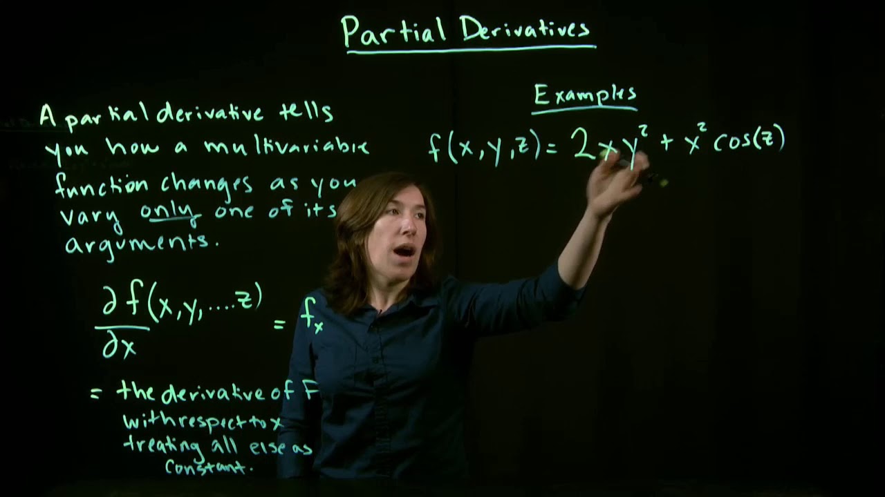
- 📉 The process of taking partial derivatives is described, where one treats all other variables as constants while differentiating with respect to one variable.
- 📌 The script clarifies the notation used for partial derivatives, which involves a 'curl' at the top of the 'd' to indicate a partial derivative, such as ∂F/∂X.
- 🤔 The reason behind the term 'partial' is explained, indicating that each partial derivative only provides a part of the full story of how the function changes.
- 📑 The script provides a step-by-step example of calculating the partial derivatives of a given function F(X, Y) = X^2 * Y + sin(Y) at a specific point (1, 2).
- 🔢 It demonstrates how to find both ∂F/∂X and ∂F/∂Y, treating Y and X as constants respectively, and then evaluates these at the given point.
- 📘 The general formula for partial derivatives is explained, showing how to differentiate the function with respect to one variable while considering the other as constant without initially substituting a specific value.
- 🔬 The script concludes by emphasizing the broader concept of derivatives beyond graphs and slopes, which is essential for understanding multi-variable calculus in higher dimensions.
Q & A
What is a multi-variable function?
-A multi-variable function is a function that takes more than one input variable, such as F(X, Y), and returns a single scalar value as output.
How is a partial derivative similar to an ordinary derivative?
-A partial derivative is similar to an ordinary derivative in that it measures the rate of change of a function with respect to one variable, treating the other variables as constants.
What is the Leibniz notation for derivatives?
-The Leibniz notation for derivatives is a way to express the derivative of a function, often written as df/dx, which suggests the change in the function (df) due to a small change in the variable (dx).
How is the derivative of a function interpreted in terms of a graph?
-In terms of a graph, the derivative of a function represents the slope of the tangent line to the curve at a particular point, which is the rate of change of the output for a small change in the input.
What does the 'D' with a curl at the top symbolize in mathematics?
-The 'D' with a curl at the top is a symbol used to denote a partial derivative, emphasizing that the derivative is being taken with respect to one variable in a multi-variable function.
Why are partial derivatives called 'partial'?
-Partial derivatives are called 'partial' because they provide only a part of the complete rate of change of a function, focusing on changes in one direction while holding other variables constant.
How do you compute the partial derivative of a function with respect to a specific variable?
-To compute the partial derivative of a function with respect to a specific variable, you treat all other variables as constants and differentiate the function as you would with an ordinary derivative.
What is the difference between computing a partial derivative at a specific point and a general formula for a partial derivative?
-Computing a partial derivative at a specific point involves substituting the values of the variables into the function and then differentiating. A general formula for a partial derivative, on the other hand, is an expression that can be used to find the derivative for any values of the variables.
How does the concept of 'nudging' the input help in understanding derivatives?
-The concept of 'nudging' the input helps in understanding derivatives by visualizing a small change in the input variable and observing the resulting change in the output, which is then used to calculate the derivative as the ratio of these changes.
What is the significance of understanding derivatives beyond just graphs and slopes?
-Understanding derivatives beyond just graphs and slopes is significant because it allows for the application of the concept to functions with higher dimensions or vector-valued functions where graphical representation is not feasible.
Outlines
📚 Introduction to Partial Derivatives
This paragraph introduces the concept of partial derivatives in the context of multi-variable functions. It begins by comparing partial derivatives to ordinary derivatives and aims to show their similarities. The speaker uses the function F(X, Y) = X^2 * Y + sin(Y) as an example and explains the notation for derivatives, including the Leibniz notation. The explanation includes a visual representation of how a small change in the input (nudge) affects the output, highlighting the concept of slope in the context of graphs. The paragraph sets the stage for understanding how to calculate partial derivatives by considering one variable at a time while treating the others as constants.
🔍 Calculating Partial Derivatives
The second paragraph delves into the actual process of calculating partial derivatives. It demonstrates how to find the partial derivative of the function F(X, Y) with respect to X and Y at a specific point (1, 2), treating the other variable as a constant. The speaker simplifies the function by substituting the constant value of the non-differentiated variable and then performs the derivative as an ordinary derivative. This results in specific values for the partial derivatives at the given point. The paragraph also discusses the general formula for partial derivatives, emphasizing the process of treating variables as constants during differentiation. The summary includes the general formulas obtained for ∂F/∂X and ∂F/∂Y, illustrating how these can be applied to any point (X, Y).
📘 Generalizing the Concept of Derivatives
The final paragraph emphasizes the broader concept of derivatives beyond the graphical representation of slopes. It explains that while graphs and slopes are useful for understanding derivatives in two dimensions, they are not applicable in higher dimensions or for vector-valued functions. The paragraph reinforces the idea of 'nudging' the input in a certain direction to see how it affects the output, and then taking the ratio of the output change to the input change as a more general approach to understanding derivatives. This approach is highlighted as essential for further studies in multi-variable calculus.
Mindmap
Keywords
💡Multi-variable function
💡Partial derivative
💡Leibniz notation
💡Graph
💡Slope
💡Input space
💡Output
💡Constant
💡Ordinary derivative
💡General formula
💡Vector-valued functions
Highlights
Introduction to multi-variable functions and the concept of partial derivatives.
Comparison between partial derivatives and ordinary derivatives, highlighting their similarities.
Explanation of the Leibniz notation for derivatives and its interpretative advantages.
Graphical representation of the derivative as the slope of a function's tangent line.
Interpretation of 'dx' as a small nudge in the x-direction and its impact on the function's output.
Illustration of how to visualize multi-variable functions in the xy-plane.
Demonstration of how to calculate the partial derivative with respect to x by treating y as a constant.
Calculation of the partial derivative with respect to y, emphasizing the constant treatment of x.
Introduction of the 'partial' notation and its significance in multi-variable calculus.
Explanation of why partial derivatives are termed 'partial' due to their focus on one variable at a time.
Step-by-step calculation of the partial derivative of F with respect to x at a specific point (1,2).
Step-by-step calculation of the partial derivative of F with respect to y at the same point (1,2).
General formula derivation for the partial derivative with respect to x, considering y as a constant.
General formula derivation for the partial derivative with respect to y, considering x as a constant.
Discussion on the importance of understanding partial derivatives beyond graphical interpretations.
Emphasis on the general approach to understanding derivatives through input and output nudges and their ratios.
Teaser for the next video, which will explore the meaning of partial derivatives in terms of graphs and slopes.
Transcripts


5.0 / 5 (0 votes)
Thanks for rating: