Calculus 1 Lecture 1.4: Continuity of Functions
TLDRThe video script delves into the concept of continuity in mathematics, particularly within the domain of functions. It explains that a function is considered continuous if it has no gaps, breaks, or asymptotes, which can be visualized as being able to draw the function without lifting the pen. The script further clarifies this with a three-point mathematical definition involving the existence of a function at a point, the existence of a limit at that point, and the equality of the function's value to the limit. The discussion encompasses various types of discontinuities, such as removable and infinite discontinuities, and how they manifest in functions. The script also explores the properties of limits and their behavior at endpoints, emphasizing the importance of one-sided limits in such cases. It concludes with an exploration of the intermediate value theorem, which states that a continuous function will take on any value between its endpoints within that interval, and demonstrates how this principle can be used to approximate roots of functions. The content is enriched with examples and applications, making it a comprehensive overview of continuity and its implications in mathematical analysis.
Takeaways
- 📐 **Continuity Definition**: A function is continuous if it has no holes, breaks, or asymptotes, meaning you can draw its graph without lifting the pen.
- 🔍 **Mathematical Continuity**: A function is continuous at a point C if it is defined at C, the limit exists at C, and the limit as X approaches C is equal to the function value at C.
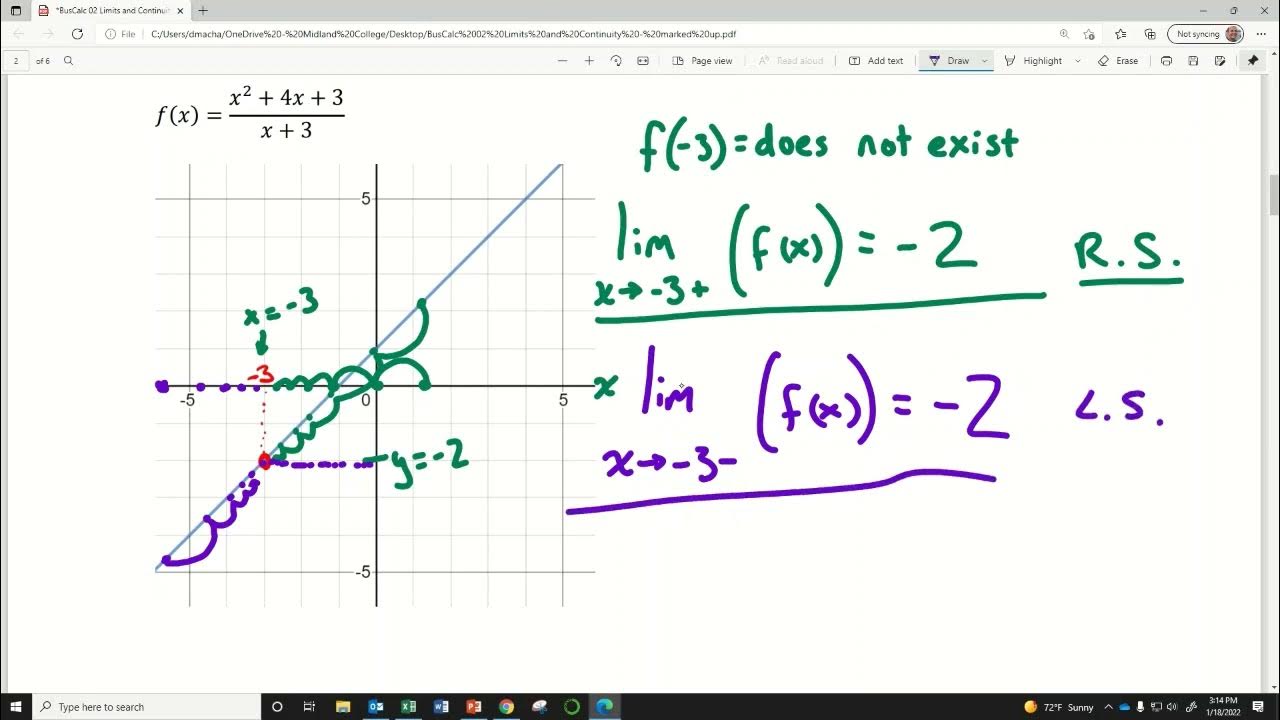
- ⚫️ **Removable Discontinuity**: A removable discontinuity is a hole in the graph that can be 'filled in' by redefining the function at that point.
- ✅ **Continuity on an Interval**: If a function is continuous at every point between two endpoints A and B, it is said to be continuous on the interval AB.
- 🔑 **One-Sided Limits**: At endpoints, a two-sided limit may not exist, so one-sided limits from the left and right are considered.
- 🔢 **Polynomial Continuity**: Every polynomial function is continuous everywhere because they can be evaluated at any point without issue.
- 🤔 **Rational Functions**: Rational functions are continuous everywhere except where the denominator is zero, which may cause a hole or an asymptote.
- 📉 **Absolute Value Continuity**: The absolute value function is continuous everywhere, as it can be defined piecewise with polynomials and constants.
- 🔄 **Composition of Functions**: If two functions are continuous everywhere, their composition will also be continuous everywhere.
- 🔮 **Intermediate Value Theorem**: For a continuous function on a closed interval, if the function values at the endpoints have different signs, there is at least one root within that interval.
- 🔍 **Root Approximation**: The intermediate value theorem can be used to approximate roots of a function by narrowing down the interval between points where the function switches from positive to negative or vice versa.
Q & A
What is the basic definition of continuity for a function?
-A function is considered continuous if it has no holes, breaks, or asymptotes. Graphically, if you can draw the function without lifting your pencil off the paper, it is continuous.
What are the three conditions for a function to be continuous at a point C?
-A function is continuous at a point C if: 1) the function is defined at that point, 2) the limit exists at that point, and 3) the value of the function at that point is equal to the limit as X approaches C.
What is a removable discontinuity?
-A removable discontinuity is a type of discontinuity where the graph of the function has a hole at a certain point, but this hole can be 'filled in' by redefining the function at that point, resulting in a continuous function.
What is an infinite discontinuity?
-An infinite discontinuity occurs when the limit of the function as it approaches a certain point is infinite. This means that the function is not defined at that point and cannot be 'filled in' to make it continuous.
How can you determine if a function is continuous on a closed interval?
-To determine if a function is continuous on a closed interval, you must check for continuity on the open interval between the endpoints and also check the one-sided limits at each endpoint to ensure they match the function's value at those points.
What is the Intermediate Value Theorem, and how is it applied?
-The Intermediate Value Theorem states that if a function is continuous on a closed interval and takes on different signs at the endpoints, then there exists at least one root within that interval. It is applied to approximate roots of a function by iteratively narrowing the interval based on the function's output signs.
Why are polynomials always continuous everywhere?
-Polynomials are always continuous everywhere because they are composed of terms with non-negative integer exponents, which means there are no breaks, holes, or asymptotes in their graph. The limit of a polynomial as X approaches any value C is simply the value of the polynomial at C.
What is a jump discontinuity?
-A jump discontinuity is a point on the graph of a function where there is an abrupt change in value, resembling a 'jump'. At this point, the function values from the left and right do not converge to a single value as X approaches the point of discontinuity.
How can you prove that the absolute value function is continuous everywhere?
-The absolute value function can be defined as a piecewise function consisting of polynomials for both the positive and negative parts and a constant for zero. Since polynomials are continuous and constants are also continuous, the absolute value function is continuous everywhere.
What is the significance of the Intermediate Value Theorem in finding the roots of a function?
-The Intermediate Value Theorem guarantees the existence of at least one root within an interval where the function values at the endpoints have different signs. This principle is crucial for root-finding algorithms, as it ensures that iterative methods will eventually converge to a root.
How does the continuity of a function affect its composition with another function?
-If two functions are continuous on their respective domains, their composition will also be continuous on the domain where the composition is defined. However, for the composition to be valid, the output of the first function must be within the domain of the second function.
Outlines
📐 Understanding Continuity in Functions
The first paragraph introduces the concept of continuity in functions. It explains that a function is considered continuous if it has no gaps, breaks, or asymptotes, meaning you can draw its graph without lifting the pencil. The mathematical definition of continuity involves three conditions: the function must be defined at a point, the limit at that point must exist, and the function's value at the point must equal the limit. This paragraph also touches on the idea of continuity over a range of points and the concept of removable discontinuities, which are gaps that can be filled with a single point.
🔍 Evaluating Continuity with Pictorial Examples
The second paragraph delves into the application of the continuity definition with visual examples. It discusses how to check for continuity at a point by ensuring the existence of the function value, the limit, and that the limit equals the function value at that point. The paragraph also explains the concept of removable discontinuities, where a hole in the function can be filled with a single point, and non-removable discontinuities, which are like jumps that cannot be filled.
🤔 Continuity and One-Sided Limits at Endpoints
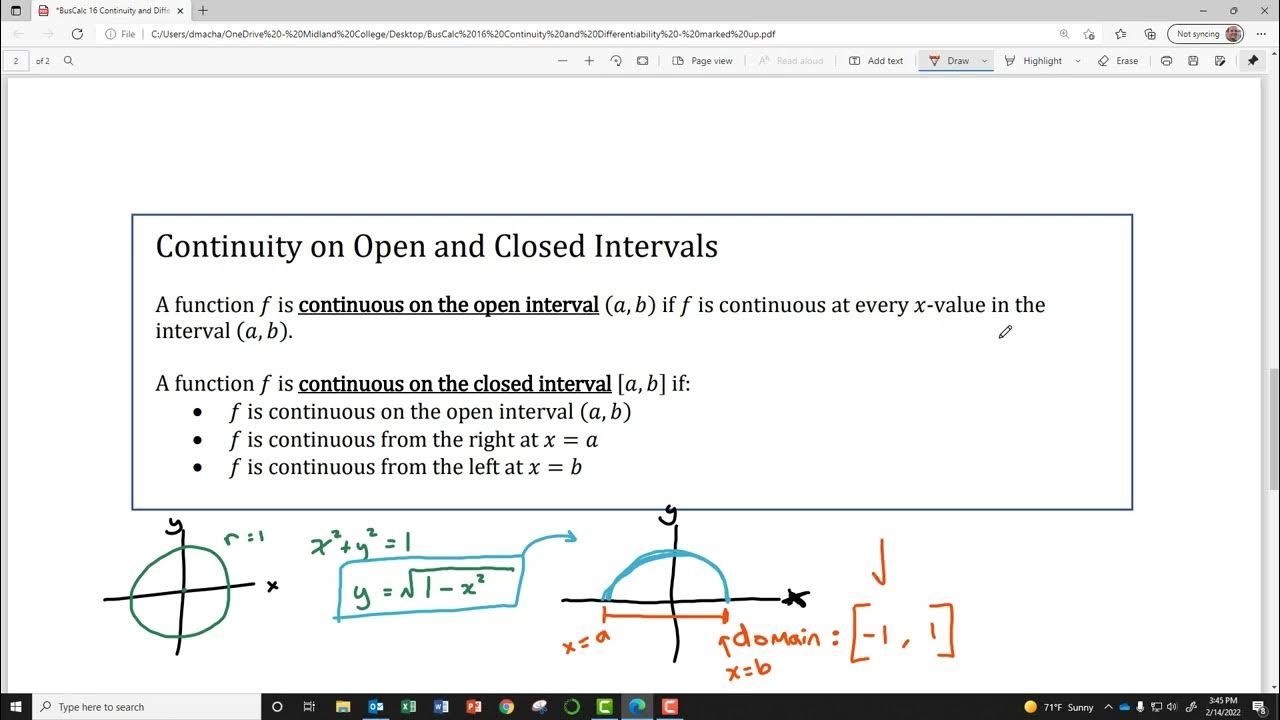
The third paragraph focuses on the nuances of continuity at endpoints of a function's domain. It clarifies that while continuity within an interval can be checked by ensuring the function's existence and the equality of the function value to the limit, endpoints require checking one-sided limits. The paragraph emphasizes that if a function is continuous at every point within an interval, it is considered continuous on that interval. However, the endpoints are only included if they satisfy the conditions of continuity from the appropriate side.
🔢 Proving Continuity Over a Closed Interval
The fourth paragraph outlines the process of proving continuity over a closed interval. It involves checking the function's continuity on the open interval between the endpoints and then verifying continuity at each endpoint separately. The paragraph explains that this requires checking one-sided limits at the endpoints and ensuring they match the function's value at those points. The process is broken down into three parts: checking the open interval, the right endpoint, and the left endpoint.
🧩 Composition of Continuous Functions
The fifth paragraph explores the properties of limits and continuity in the context of composite functions. It establishes that if two functions are continuous at a point, their sum, difference, and product are also continuous at that point. However, division requires the additional condition that the denominator is not zero at that point to ensure continuity. The paragraph also touches on the concept of one-sided limits and how they relate to continuity at endpoints.
📉 Continuity and Polynomial Functions
The sixth paragraph discusses the relationship between polynomial functions and continuity. It states that since polynomials can be evaluated by simply plugging in the value of x (due to their being composed of terms with non-negative integer exponents), every polynomial function is continuous everywhere. This leads to the conclusion that rational functions, which are ratios of polynomials, are also continuous everywhere except where the denominator equals zero, which would result in a discontinuity.
🔍 Identifying Discontinuities in Rational Functions
The seventh paragraph provides a method for identifying discontinuities in rational functions. It explains that discontinuities occur where the denominator equals zero and that factoring the numerator and denominator can help determine the nature of the discontinuity. If a discontinuity can be 'crossed out' by factoring, it is a removable discontinuity (a hole). If not, it is an asymptote. The paragraph also emphasizes that one cannot simply eliminate discontinuities without proper justification.
🔁 Continuity of the Absolute Value Function
The eighth paragraph focuses on proving the continuity of the absolute value function. It breaks down the absolute value function into two cases (for x greater than zero and for x less than zero) and shows that at the point where x equals zero, the one-sided limits exist and are equal. This fulfills the criteria for continuity, proving that the absolute value function is continuous everywhere.
🎼 Compositions and Inverse Functions
The ninth paragraph discusses the continuity of compositions and inverse functions. It states that if two functions are continuous everywhere, their composition will also be continuous everywhere. Additionally, if a function is continuous on its domain, its inverse will be continuous on its domain, with the caveat that the domain of the inverse function is the range of the original function.
🔍 Intermediate Value Theorem
The tenth paragraph introduces the Intermediate Value Theorem, which states that if a function is continuous on a closed interval and takes on different signs at the endpoints, then there exists at least one root within that interval. The theorem is particularly useful for approximating roots of functions, as it guarantees the existence of a point that maps to a given value within a specified range of the function's outputs.
🔢 Approximating Roots Using IVT
The eleventh paragraph provides a practical application of the Intermediate Value Theorem for approximating roots of functions. It describes a method for narrowing down the location of a root by evaluating the function at intervals and observing the sign changes of the results. This iterative process allows for increasingly accurate approximations of the root's location.
📝 Manual Calculation of Roots
The twelfth paragraph offers a manual approach to finding roots without the aid of calculators or computers. It involves creating a table of values and iteratively refining the interval within which a root is known to exist based on the function's output signs. This method, while time-consuming, can achieve a high degree of accuracy and provides a deeper understanding of the function's behavior.
Mindmap
Keywords
💡Continuity
💡Removable Discontinuity
💡Jump Discontinuity
💡Infinite Discontinuity
💡One-Sided Limits
💡Polynomial Functions
💡Rational Functions
💡Asymptotes
💡Intermediate Value Theorem
💡Roots of a Function
💡Composition of Functions
Highlights
A function is considered continuous if it has no holes, breaks, or asymptotes, allowing for a graph to be drawn without lifting the pencil.
Mathematically, a function is continuous at a point C if it is defined at that point, the limit exists at that point, and the limit equals the function value.
Removable discontinuities are points where the function can be redefined to fill in a hole, making the function continuous at that point.
A jump discontinuity occurs when the function jumps from one value to another, and it cannot be filled in with a single point.
An infinite discontinuity happens when the function's value or limit tends to infinity at a certain point.
Rational functions are continuous everywhere except where the denominator equals zero, which would result in a discontinuity.
Every polynomial is continuous everywhere because polynomials can be evaluated by simply plugging in the value of x.
For a function to be continuous on a closed interval, it must be continuous on the open interval between the endpoints and at each endpoint.
The Intermediate Value Theorem states that if a function is continuous on a closed interval and the function values at the endpoints have different signs, there is at least one root within that interval.
The theorem can be used to approximate roots of a function by iteratively narrowing the interval where the root must lie based on the function values' signs.
If two functions are continuous everywhere, their composition will also be continuous everywhere.
The continuity of a function allows for the application of various theorems and properties that can simplify the analysis of the function's behavior.
The concept of continuity is fundamental in calculus and is used to define other concepts such as limits, derivatives, and integrals.
Understanding discontinuities is crucial for the analysis of a function's graph, as they represent points where the graph has breaks, jumps, or tends to infinity.
The properties of limits and continuity can be applied to rational functions to determine their behavior at points where the denominator is zero.
The Intermediate Value Theorem is a powerful tool for approximating the roots of a continuous function without the need for complex calculations or technology.
Continuous functions have real-world applications in fields such as physics and engineering, where they can model phenomena that change smoothly over time.
Transcripts


5.0 / 5 (0 votes)
Thanks for rating: