Least squares | MIT 18.02SC Multivariable Calculus, Fall 2010
TLDRIn this educational video, the presenter explains the least squares method for fitting a line to a set of three data points. The method aims to minimize the sum of the squares of the vertical distances from the data points to the line. The presenter demonstrates the process of setting up and solving a system of linear equations to find the best-fit line's slope and intercept. Additionally, the video introduces the concept of fitting higher-degree polynomials, such as a parabola, to the data for a more sophisticated model, highlighting the process of optimization and the use of partial derivatives to find the best-fit parameters.
Takeaways
- 📈 The goal of the least squares method is to fit a line to a set of data points by minimizing the sum of the squares of the vertical distances (residuals) between the data points and the line.
- 🔍 The problem provided involves fitting a line to three data points: (0, 1), (2, 1), and (3, 4), with the objective of minimizing the squared differences between the actual and expected y-values.
- 📊 To visually understand the process, a rough graph of the data points is drawn, and an initial guess for the least squares line is made.
- 🧠 The concept of minimizing the area of squares formed by the differences between the expected and actual y-values is introduced as the method to find the optimal line.
- 📝 The script outlines the mathematical process, which involves setting up a system of equations based on the sum of x-values, y-values, x-squared values, and x*y product from the data points.
- 🔢 The values calculated from the data points are: the sum of x_i's is 5, the sum of y_i's is 6, the sum of x_i squared is 13, and the sum of x_i*y_i product is 14.
- 🏁 The system of equations to be solved is: 13a + 5b = 14 and 5a + 3b = 6, where 'a' represents the slope and 'b' the y-intercept of the line.
- 📱 The solution to the system of equations yields the slope (a) as 6/7 and the y-intercept (b) as 4/7, resulting in the least squares line equation y = 6/7x + 4/7.
- 🚀 The script also mentions the possibility of fitting higher-degree polynomials, such as a parabola, to the data points using a similar least squares approach.
- 📚 For the challenge problem, the function to be minimized in the case of fitting a parabola becomes y_i - (a x_i^2 + b x_i + c)^2, where 'a', 'b', and 'c' are the coefficients to be determined.
- 💡 The process of solving for the coefficients of the parabola involves taking partial derivatives of the function with respect to 'a', 'b', and 'c', setting them to zero, and solving the resulting system of three equations with three unknowns.
Q & A
What is the main objective of using least squares in this context?
-The main objective of using least squares in this context is to fit a line to a set of data points by minimizing the sum of the squares of the vertical distances (residuals) between the data points and the fitted line.
What are the three data points given in the transcript for fitting the line?
-The three data points given are (0, 1), (2, 1), and (3, 4).
What does the term 'expected value' refer to in the context of least squares?
-In the context of least squares, the 'expected value' refers to the value predicted by the model (in this case, the line) for a given x-value. It is the value on the line that corresponds to the actual data point's x-coordinate.
What is the formula for the least squares line?
-The formula for the least squares line is y = mx + b, where m is the slope of the line and b is the y-intercept.
How are the slope (m) and y-intercept (b) of the least squares line calculated?
-The slope (m) and y-intercept (b) are calculated by solving a system of linear equations derived from the least squares minimization problem. These equations are derived by setting the partial derivatives of the sum of squared residuals with respect to m and b equal to zero and solving for m and b.
What are the values of the slope (m) and y-intercept (b) for the given data points?
-For the given data points, the slope (m) is 6/7 and the y-intercept (b) is 4/7.
What is the equation of the least squares line for the given data points?
-The equation of the least squares line for the given data points is y = (6/7)x + (4/7).
How does the least squares method differ from other curve fitting techniques?
-The least squares method specifically fits the best straight line to a set of data points by minimizing the sum of squared residuals. Other curve fitting techniques, such as fitting a higher-degree polynomial or a parabola, involve different objective functions and potentially more complex optimization problems.
What is the challenge problem mentioned at the end of the transcript?
-The challenge problem mentioned at the end of the transcript is to use the least squares method to fit a parabola (a quadratic function) to the given data points instead of a straight line.
How many equations and unknowns are in the system derived from the least squares method for a straight line?
-There are two equations and two unknowns in the system derived from the least squares method for a straight line, one for the slope (m) and one for the y-intercept (b).
What is the significance of minimizing the sum of squared residuals in the least squares method?
-Minimizing the sum of squared residuals ensures that the fitted line is as close as possible to all the data points, on average. This is a way to find the best approximation of the data with a straight line, considering all data points equally important.
Outlines
📈 Introduction to Least Squares Method
In this introductory section, Christine Breiner welcomes the audience back to recitation and outlines the task at hand: using the least squares method to fit a line to a given set of three data points (0, 1), (2, 1), and (3, 4). She encourages the audience to attempt the problem first, based on the techniques learned in class, and then return to the video for a detailed explanation and comparison of solutions. Breiner then explains the concept of least squares, emphasizing the goal of minimizing the sum of the squares of the differences between the actual and expected values. She visually describes this process on a graph, highlighting the trade-off between the sizes of the squares formed by the differences in values. The explanation progresses to discuss how adjusting the line's slope and intercept affects the sum of the areas of these squares, which is the quantity being minimized. Breiner also touches on the optimization process involving both the slope and y-intercept, which is why it's studied in multivariable calculus rather than single-variable calculus. Finally, she presents the equations derived from optimizing the least squares line and explains the values needed for the calculation, which are the sums of the x-values, y-values, x-squared values, and x*y product from the given data points.
🧮 Solving the Least Squares System of Equations
In this segment, Breiner continues the discussion on least squares by diving into the specifics of solving the system of equations derived from the method. She presents the two equations that result from setting the partial derivatives of the function with respect to the variables (a and b) equal to zero. The equations, which involve the sums of the x_i's, y_i's, x_i squared, and x_i*y_i product from the data points, are used to solve for the slope (a) and the y-intercept (b). Breiner calculates the values of a and b, finding them to be 6/7 and 4/7, respectively. This leads to the equation of the least squares line, y = (6/7)x + 4/7, which is the best fit for the given data points. She concludes this part by hinting at a more advanced application of least squares for fitting higher-degree polynomials, such as a parabola, to the data. Breiner outlines the function form for the challenge problem, which involves minimizing a different function that accounts for the squared differences between the actual and expected values based on a quadratic equation. She explains the process of taking partial derivatives with respect to each variable (a, b, and c) and setting them to zero to solve for the coefficients of the quadratic equation, which will give the parabola of best fit for the three data points.
Mindmap
Keywords
💡Least Squares
💡Line of Best Fit
💡Slope (a)
💡Y-Intercept (b)
💡Residuals
💡Optimization
💡Derivative
💡System of Equations
💡Polynomial
💡Parabola
💡Multivariable Calculus
Highlights
The video introduces the concept of using least squares to fit a line to a set of data points.
Three specific data points are given: (0, 1), (2, 1), and (3, 4).
A rough picture of the data points on a graph is mentioned to provide a visual context.
The goal of least squares is to minimize the difference between the actual and expected values, squared.
The process involves finding the line that minimizes the sum of the areas of squares representing the differences between actual and expected values.
The video explains that optimizing the line involves finding the best y-intercept and slope simultaneously.
The equations for optimizing the least squares line are derived by taking derivatives with respect to the variables and setting them to zero.
The sum of x values is calculated as 5, the sum of y values as 6, the sum of x squared values as 13, and the sum of x*y product as 14.
The system of equations to solve for the least squares line is presented as 13a + 5b = 14 and 5a + 3b = 6.
The solution to the system of equations yields a slope (a) of 6/7 and a y-intercept (b) of 4/7.
The least squares line is expressed as y = 6/7x + 4/7.
The video mentions a challenge problem where a higher-degree polynomial, such as a parabola, can be fit to the data.
The function to be minimized for fitting a parabola is described, involving three variables a, b, and c.
The process for fitting a parabola involves taking partial derivatives with respect to each variable, setting them to zero, and solving the resulting system of equations.
The video concludes by encouraging viewers to attempt the challenge problem of finding the quadratic of best fit for the given data points.
Transcripts
Browse More Related Video
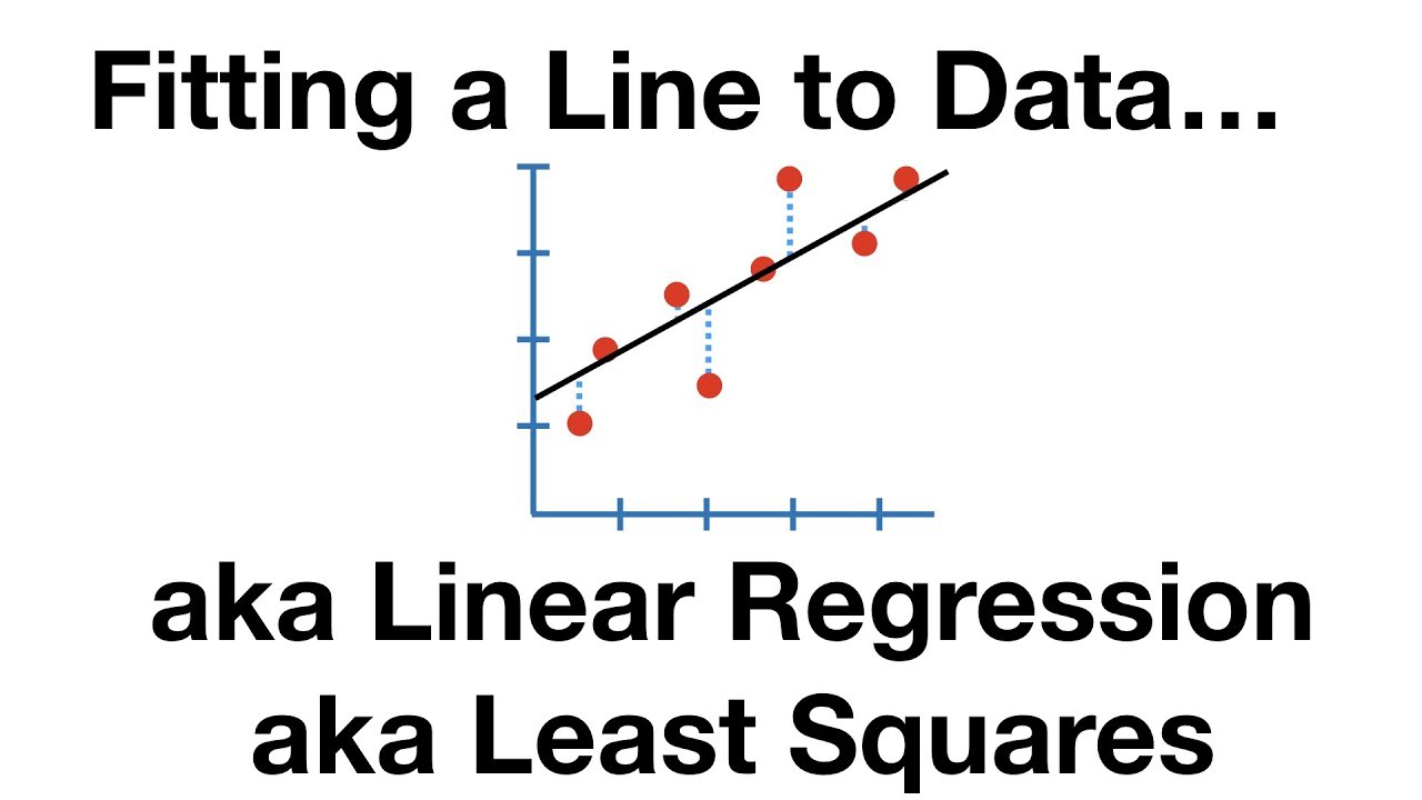
The Main Ideas of Fitting a Line to Data (The Main Ideas of Least Squares and Linear Regression.)

Lec 9: Max-min problems; least squares | MIT 18.02 Multivariable Calculus, Fall 2007

Calculus Chapter 2 Lecture 14 BONUS

Introduction To Ordinary Least Squares With Examples
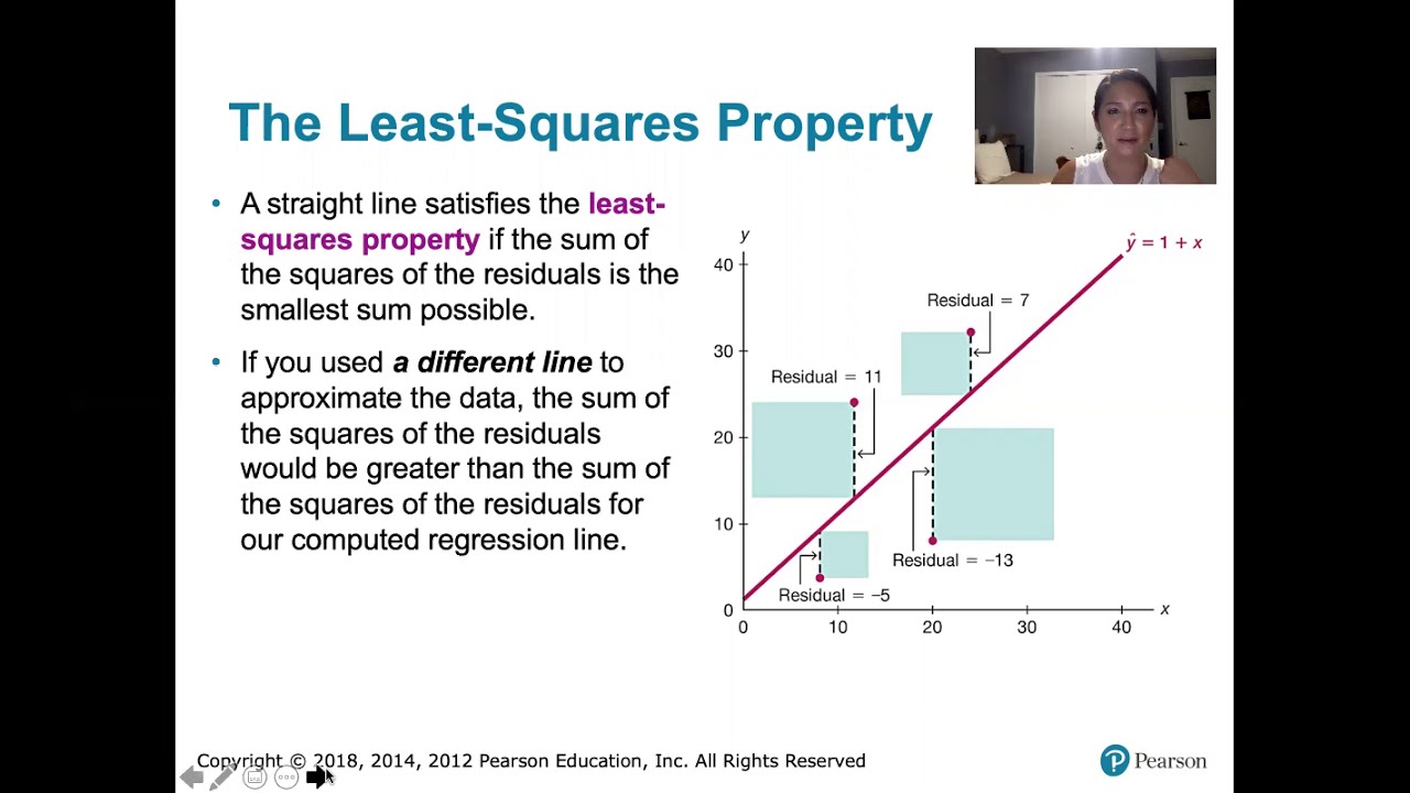
10.2.5 Regression - Residuals and the Least-Squares Property
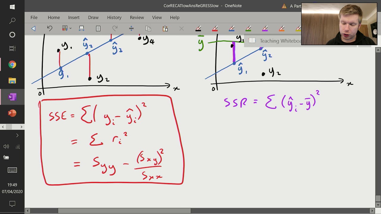
Correlation and Regression (6 of 9: Sum of Squares - SSE, SSR and SST)
5.0 / 5 (0 votes)
Thanks for rating: