Lec 9: Max-min problems; least squares | MIT 18.02 Multivariable Calculus, Fall 2007
TLDRThis script from an MIT OpenCourseWare lecture delves into the application of partial derivatives in solving multivariable minimization and maximization problems. It explains the concept of partial derivatives, the tangent plane approximation, and how to identify critical points as potential minima, maxima, or saddle points. The lecture also touches on the least-squares method for data fitting, illustrating how to find the best fit line for a given set of data points by minimizing the sum of squared errors, and extends the concept to exponential and quadratic fits.
Takeaways
- 📚 The lecture discusses the application of partial derivatives to solve minimization and maximization problems involving functions of multiple variables.
- 🔍 Partial derivatives, such as ∂f/∂x and ∂f/∂y, represent the rate of change of a function with respect to one variable while keeping the other constant.
- 📈 The approximation formula for the change in a function when both variables are varied is given by ∆z ≈ (∂f/∂x)∆x + (∂f/∂y)∆y, highlighting the additive effects of small changes in multiple variables.
- 📐 The tangent plane approximation is introduced as a method to understand the behavior of a function near a point, with the tangent plane being determined by the slopes of tangent lines in the x and y directions.
- 🔑 Critical points are defined as points where all partial derivatives are zero, which are potential candidates for local minima, local maxima, or saddle points.
- 🔄 The process of finding critical points involves setting the first partial derivatives to zero and solving the resulting system of equations.
- 📉 The script provides an example of a function f(x, y) and demonstrates how to find its critical point by setting the partial derivatives equal to zero and solving for x and y.
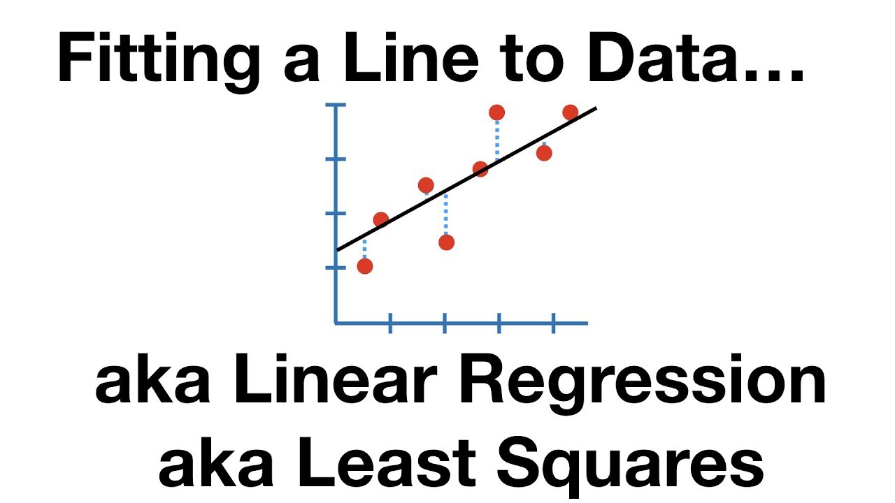
- 📊 Least-squares fitting is introduced as a method to find the 'best fit' line or curve for a given set of data points, which is a common task in experimental sciences.
- ⚖️ The least-squares method minimizes the sum of the squares of the deviations between the observed data and the values predicted by the model.
- 📐 The process of finding the best fit involves taking partial derivatives of the error function with respect to the parameters of the model and solving for when these derivatives are zero.
- 🔍 The script also discusses how to handle different types of models for best fit, such as linear, exponential, and quadratic, by transforming the problem into a linear system of equations that can be solved.
Q & A
What is the purpose of MIT OpenCourseWare and how can one support it?
-MIT OpenCourseWare aims to offer high-quality educational resources for free. Support can be provided through donations or by viewing additional materials from various MIT courses on their website at ocw.mit.edu.
What is the significance of partial derivatives in the context of the script?
-Partial derivatives are used to handle minimization or maximization problems involving functions of several variables. They measure the rate of change of a function with respect to one variable while keeping the others constant.
What is the approximation formula for changes in a function of two variables when both variables are varied?
-The approximation formula states that if a function z = f(x, y) is changed by small amounts delta x and delta y, then the change in the function, delta z, is approximately equal to (∂f/∂x) * delta x + (∂f/∂y) * delta y.
How does the tangent plane approximation relate to the partial derivatives of a function?
-The tangent plane approximation is used to justify the partial derivative formula. It is based on the idea that the graph of a function is close to its tangent plane, especially for small changes in the variables. The slopes of the tangent lines to the surface, which are the partial derivatives, help determine the tangent plane.
What is the condition for a point to be considered a critical point of a function of two variables?
-A point (x0, y0) is considered a critical point of a function f if both partial derivatives, ∂f/∂x and ∂f/∂y, are zero at that point. This implies that the function does not change to the first order in either variable.
Why are both partial derivatives being zero necessary for a local minimum or maximum?
-Both partial derivatives being zero ensures that the function does not change to the first order when either variable is varied. If only one partial derivative is zero, the function could still change when the other variable is adjusted, so it would not represent a true local minimum or maximum.
How can the second derivative test be used to determine the nature of a critical point?
-The second derivative test involves analyzing the second partial derivatives and the Hessian matrix to determine if a critical point is a local minimum, local maximum, or a saddle point. This will be covered in more detail in subsequent lectures.
What is the least-squares fitting and why is it used in experimental sciences?
-Least-squares fitting is a method used to find the 'best fit' line or curve for a set of data points by minimizing the sum of the squares of the errors. It is used in experimental sciences to model and predict relationships between variables based on collected data.
How does the process of least-squares fitting relate to the minimization of a function?
-Least-squares fitting is a specific application of minimization where the function to be minimized is the sum of the squares of the deviations between the observed data and the predicted values from the model. The minimization is achieved by finding the coefficients that result in the smallest total square error.
What is Moore's law and how does it relate to the concept of best fit in the script?
-Moore's law is the observation that the number of transistors on a computer chip doubles approximately every two years, often associated with an exponential growth in computing power. The script uses Moore's law as an example to illustrate how an exponential fit, rather than a linear one, can be the best fit for certain types of data.
How can one find the best exponential fit for a set of data points?
-To find the best exponential fit, one can take the logarithm of the y-values and then perform a linear least-squares fit on the log-transformed data. The parameters of the exponential fit can then be determined from the slope and intercept of this linear fit.
What is the significance of the least-squares method in fitting various types of models to data?
-The least-squares method is significant because it provides a systematic way to find the best fit for different types of models, such as linear, exponential, or quadratic, by minimizing the total square deviation between the model predictions and the actual data points.
Outlines
📚 Introduction to Partial Derivatives and Optimization
This paragraph introduces the concept of partial derivatives and their application in optimization problems involving functions of multiple variables. It explains how partial derivatives, such as partial f with respect to x (f_x) and partial f with respect to y (f_y), are used to measure the rate of change of a function when one variable is changed while keeping the other constant. The approximation formula for the change in a function when both variables are varied is discussed, highlighting its importance in understanding the behavior of multivariable functions. The tangent plane approximation is introduced as a method to justify the approximation formula, providing a geometric interpretation of partial derivatives.
📐 Tangent Plane Approximation and Its Implications
The paragraph delves deeper into the tangent plane approximation, explaining how the slopes of the tangent lines to the graph of a function in the x and y directions determine the tangent plane. The equations of these tangent lines are derived, and it is shown how they combine to form the equation of the tangent plane. The paragraph also discusses how the graph of a function closely approximates its tangent plane, especially for small changes in x and y, and how this approximation can be used to estimate changes in the function's value. The concept is further clarified with the idea that if both partial derivatives are zero, the tangent plane is horizontal, indicating a potential maximum or minimum.
🔍 Critical Points and Their Significance in Optimization
This section focuses on the concept of critical points in multivariable functions, where both partial derivatives are zero. It explains the necessity of this condition for a point to be considered a local minimum or maximum. The importance of having both partial derivatives being zero simultaneously is discussed, as it ensures that the function does not change to the first order when either variable is perturbed. The paragraph also introduces the idea that not all points where partial derivatives are zero are minima or maxima, and that further analysis is required to classify them.
🧩 Example Analysis and Simplification of a Given Function
The paragraph presents an example function and guides through the process of finding its critical points by setting the partial derivatives to zero. It emphasizes the importance of maintaining two separate equations when solving for the variables. The example demonstrates how to simplify the equations and solve for the critical point, which in this case is found to be (-1, 0). The discussion also touches on the challenge of determining whether a critical point is a maximum, minimum, or saddle point, with a promise to address this in the next session.
🤔 Completing the Square and Identifying the Nature of Critical Points
This paragraph continues the discussion on the example function by attempting to express it as a sum of squares, which simplifies the process of identifying the nature of the critical point. The speaker completes the square for the given function and shows that the critical point corresponds to the minimum value of the function. The method of completing the square is illustrated, and it is noted that while this approach was successful for the example, more general methods will be discussed in future sessions.
📉 Application of Minimization in Least Squares Fitting
The paragraph introduces the application of minimization in the context of least squares fitting, a common technique in experimental sciences. It discusses how to find the 'best fit' line for a set of data points, emphasizing that the goal is to minimize the total square error between the observed data and the predicted values from the line. The paragraph also touches on the limitations of using such models for unpredictable phenomena like the stock market.
📊 Deriving the Best Fit Line Using Least Squares Method
This section provides a detailed explanation of how to derive the best fit line using the least squares method. It discusses setting up the error function and finding its critical points by taking partial derivatives with respect to the coefficients of the line. The process of simplifying the equations to form a linear system that can be solved for the coefficients is outlined. The paragraph also explains why this method results in a minimum error, although the detailed justification is reserved for a future session.
📈 Generalizing Least Squares to Exponential and Quadratic Fits
The final paragraph extends the concept of least squares fitting to more complex relationships beyond linear, such as exponential and quadratic fits. It uses Moore's law as an example to illustrate how an exponential fit can be determined by linearizing the problem through a logarithmic transformation. The paragraph also briefly mentions how to approach fitting a quadratic function to data, which involves setting up and solving a three-by-three linear system for the coefficients.
Mindmap
Keywords
💡Partial Derivatives
💡Tangent Plane Approximation
💡Critical Points
💡Minimization and Maximization Problems
💡Second Derivative Test
💡Least Squares
💡Linear Regression
💡Exponential Fit
💡Quadratic Law
💡Sum of Squares
Highlights
Introduction to using partial derivatives for minimization or maximization problems involving functions of several variables.
Explanation of partial derivatives as the rate of change of a function with respect to one variable while keeping the other constant.
The approximation formula for changes in a function when varying both variables, f(x, y).
The tangent plane approximation as a method to justify the partial derivative formula.
Derivation of the tangent plane equation using the slopes of tangent lines to the surface.
Understanding the tangent plane as an approximation of the function's graph near the tangent plane.
Application of partial derivatives to optimization problems in real-world scenarios such as cost minimization or profit maximization.
Condition for a local minimum or maximum where both partial derivatives are zero simultaneously.
The concept of a critical point in functions of multiple variables.
Example problem involving the function f(x, y) = x^2 - 2xy + 3y^2 + 2x - 2y and finding its critical point.
Technique of completing the square to simplify and analyze functions for minimization or maximization.
Differentiation between local minima, local maxima, and saddle points in multivariable functions.
The least-squares method for fitting a line to experimental data and its significance in scientific research.
Process of defining the 'best fit' line by minimizing the sum of squared errors.
Solving for the coefficients of the best fit line using a system of linear equations derived from the least-squares method.
Generalization of least-squares fitting to other types of relations beyond linear, such as exponential or quadratic fits.
Practical example of applying least-squares fitting to Moore's law data to determine the relation between the number of transistors and time.
The importance of understanding the nature of critical points and the conditions for minima and maxima in multivariable calculus.
Transcripts
Browse More Related Video
The Main Ideas of Fitting a Line to Data (The Main Ideas of Least Squares and Linear Regression.)

Least squares | MIT 18.02SC Multivariable Calculus, Fall 2010

Second partial derivative test

Calculus Chapter 2 Lecture 14 BONUS

Multivariable maxima and minima

Lec 10: Second derivative test; boundaries & infinity | MIT 18.02 Multivariable Calculus, Fall 2007
5.0 / 5 (0 votes)
Thanks for rating: