Calculus Chapter 2 Lecture 14 BONUS
TLDRIn this calculus lecture, Professor Greist introduces a statistical problem involving the determination of a linear relationship's slope (M) from noisy data points. The method of least squares is presented as an optimization technique to find the best fit line. The process involves minimizing the squared vertical distances between data points and the line. The derivative of the sum of these distances with respect to M is calculated to find the optimal slope. The lecture also touches on extending this approach to include a y-intercept, hinting at the complexities of multivariable calculus and its applications in fields like game theory, linear programming, and machine learning.
Takeaways
- 📚 The lecture introduces a method to determine the value of 'M' in a linear relationship between X and Y values from an experiment.
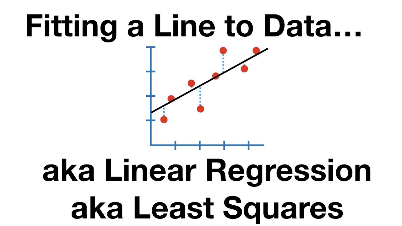
- 📈 The method of least squares is presented as a principled approach to fit a line to data points with noise.
- 🔍 The vertical distance between data points and the line is considered, and its square is used to avoid dealing with signed distances.
- 📉 The objective is to minimize the sum of the squared vertical distances, which represents the deviation of the data from the line.
- 🧐 The derivative of the deviation function with respect to 'M' is calculated to find the critical point that minimizes the deviation.
- 🔄 The derivative involves terms that are linear in 'M', which simplifies the process of finding the minimum.
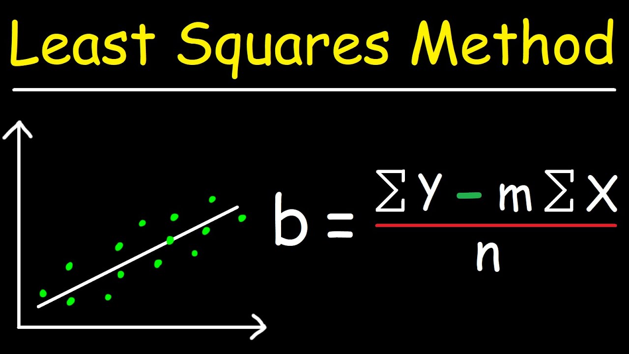
- 📝 By setting the derivative equal to zero, an equation is derived to solve for 'M' in terms of the sums of products and squares of X and Y values.
- 📉 The second derivative test is used to confirm that the critical point found is indeed a minimum by showing it is positive for all X values.
- 🤔 The script raises the question of extending this method to find the optimal 'B' in a line equation y = MX + B, which involves multivariate calculus.
- 🌐 The discussion hints at broader applications of optimization in fields like game theory, linear programming, and machine learning.
- 🌟 The importance of understanding single-variable calculus as foundational knowledge for tackling more complex optimization problems is emphasized.
Q & A
What is the main topic of Professor Greist's lecture 14?
-The main topic of the lecture is the method of least squares, an optimization technique used to determine the best-fit line for a set of data points in a linear regression problem.
Why might one need to find the value of M in a linear relationship between X and Y values?
-One might need to find the value of M to understand the slope of the best-fit line that represents the relationship between X and Y values, which can be crucial in various applications such as physical experiments or statistical analysis.
What is the issue with simply drawing a line to fit the data points?
-Drawing a line to fit the data points can be subjective and imprecise. It lacks a principled approach and does not guarantee the best fit according to any mathematical criteria.
What is the least squares method and how does it help in finding the optimal value of M?
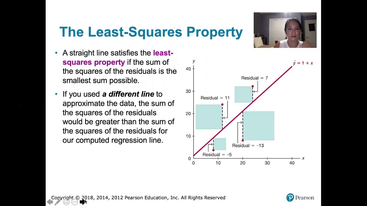
-The least squares method is a statistical technique that minimizes the sum of the squares of the vertical distances between the data points and the line of slope M. It helps in finding the optimal value of M by systematically reducing the overall deviation of the data from the line.
How does the vertical distance between the data points and the line of slope M affect the optimization problem?
-The vertical distance, represented by \( Y_i - M \times X_i \), is squared and summed up to form a function of M. The goal is to minimize this function to find the best-fit line, which is achieved by adjusting the value of M.
What is the purpose of squaring the vertical distance in the least squares method?
-Squaring the vertical distance ensures that all distances are positive and allows for the use of calculus to find the minimum value of the sum, as it is easier to differentiate and work with squared terms.
How does the derivative of the function s with respect to M help in finding the optimal M?
-The derivative of the function s with respect to M provides the rate of change of s. By setting this derivative equal to zero, we find the critical point, which is the value of M that minimizes the deviation s.
What is the significance of the second derivative test in this context?
-The second derivative test is used to determine whether the critical point found is a minimum or maximum. A positive second derivative indicates that the critical point is a local minimum, confirming that the value of M found does indeed minimize the deviation.
What happens if the line we are looking for does not pass through the origin?
-If the line does not pass through the origin, an additional parameter, the y-intercept B, is introduced. This extends the problem to finding both the slope M and the y-intercept B, which requires a multivariable optimization approach.
How does the introduction of the y-intercept B change the optimization problem?
-The introduction of B changes the optimization problem from a single-variable to a multivariable problem. It requires considering both M and B in the function s, leading to a more complex optimization process that may involve partial derivatives and techniques from multivariable calculus.
What are some fields that rely on the intuition developed from single-variable calculus for optimization?
-Fields such as game theory, linear programming, and machine learning rely on the intuition developed from single-variable calculus, particularly for finding maxima, minima, and other critical points in multivariate functions.
Outlines
📚 Introduction to Least Squares in Calculus
This paragraph introduces the concept of the least squares method in the context of a statistical problem. Professor Greist begins by presenting a scenario where an experiment yields data points that suggest a linear relationship between X and Y values, but the exact value of the proportionality constant M is unknown. The paragraph explains the need for a systematic approach to determine M, rather than a subjective one. It then outlines the least squares method as an optimization problem, where the goal is to minimize the sum of the squared vertical distances between the data points and the line with slope M. The process involves squaring the distances to avoid dealing with negative values and summing them to find the deviation from the line. The paragraph concludes with the differentiation of the deviation function with respect to M to find its minimum, which gives the optimal value of M.
🔍 Analyzing the Optimal Slope and Extending to Intercept
In this paragraph, the discussion continues with the method to determine if the critical point found for M is indeed a minimum, by examining the second derivative of the deviation function with respect to M. It is shown that the second derivative is positive, indicating a local minimum, thus confirming that the derived value of M minimizes the deviation and provides the best fit line. The paragraph then extends the discussion to cases where the line does not pass through the origin, introducing the need to also find the y-intercept B. The paragraph highlights the complexity that arises when optimizing a function with multiple variables, such as M and B, and alludes to the broader applications of such optimization problems in fields like game theory, linear programming, and machine learning. It emphasizes the importance of the intuition developed in single-variable calculus for tackling these more complex scenarios.
Mindmap
Keywords
💡Calculus
💡Linear Relationship
💡Optimization Problem
💡Least Squares
💡Data Points
💡Derivative
💡Critical Point
💡Second Derivative
💡Best Fit Line
💡Y-Intercept
💡Multivariable Calculus
Highlights
Introduction to a more involved example in calculus, motivated by a problem in statistics.
Describing a scenario where you measure X and Y values with a linear relationship but unknown constant M.
The challenge of determining the appropriate value of M when given noisy data points.
Introduction to the method of least squares as a principled approach to optimize M.
Formulating the problem as an optimization problem to minimize the deviation of data from the line of slope M.
Explanation of squaring the vertical distance to handle signed distances in the optimization function.
Derivation of the derivative of the deviation function with respect to M to find the critical point.
Simplification of the derivative to solve for M by setting it equal to zero.
The formula for calculating M as the sum of X times Y divided by the sum of X squared.
Discussion on whether the critical point is a local minimum and how to verify it.
Calculation of the second derivative to confirm the nature of the critical point.
Insight that the second derivative is non-negative, indicating a minimum.
Introduction of the possibility of the line not passing through the origin, adding complexity to the problem.
Extension of the optimization problem to include both slope M and y-intercept B.
Introduction to multivariable calculus for optimization problems with more than one input.
Mention of fields like game theory, linear programming, and machine learning that rely on optimization of multivariate functions.
Emphasis on the importance of the intuition gained from single variable calculus for future studies.
Transcripts
Browse More Related Video
The Main Ideas of Fitting a Line to Data (The Main Ideas of Least Squares and Linear Regression.)

Least squares | MIT 18.02SC Multivariable Calculus, Fall 2010

Lec 9: Max-min problems; least squares | MIT 18.02 Multivariable Calculus, Fall 2007
10.2.5 Regression - Residuals and the Least-Squares Property

Introduction To Ordinary Least Squares With Examples
Linear Regression Using Least Squares Method - Line of Best Fit Equation
5.0 / 5 (0 votes)
Thanks for rating: