The Sampling Distribution of the Sample Mean
TLDRThe video script discusses the sampling distribution of the sample mean, X bar, highlighting its two key characteristics: the mean of X bar equals the population mean, and the standard deviation of X bar equals the population standard deviation divided by the square root of the sample size. It explains how the distribution becomes more concentrated around the population mean as sample size increases, which is crucial for precise estimation. The central limit theorem is briefly introduced, noting its significance in approximating the normality of the sample mean even from non-normal distributions, provided the sample size is large. The video also touches on the concept of standardizing random variables for probability calculations and the importance of sampling distributions in statistical inference.
Takeaways
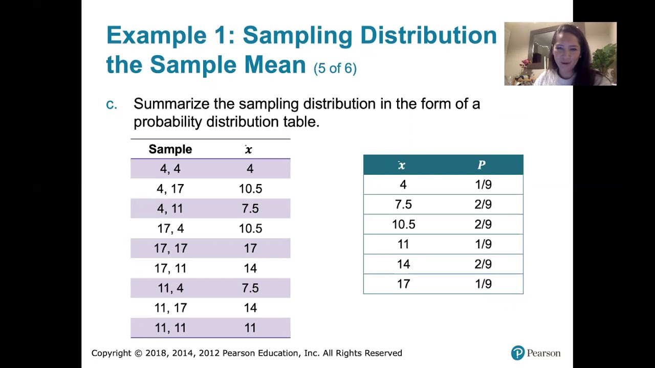
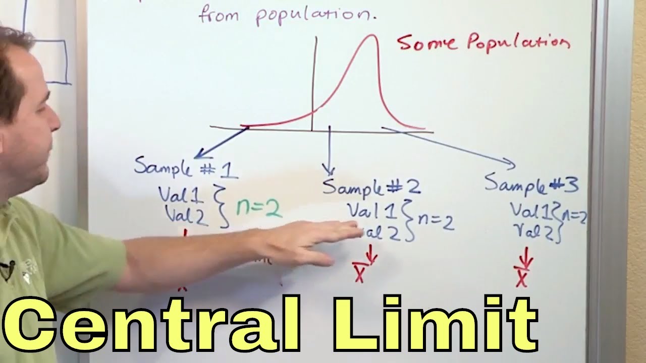
- 📈 The sampling distribution of the sample mean (X bar) is a probability distribution that describes the variation in sample means from a population.
- 🎯 Each sample mean (X bar) is a random variable that depends on the particular sample drawn from the population.
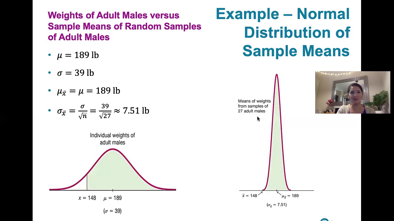
- 🌟 The mean (mu sub X bar) of the sampling distribution of X bar is equal to the mean (mu) of the population from which the sample is drawn.
- 📊 The standard deviation (sigma sub X bar) of the sampling distribution of X bar is the standard deviation (sigma) of the population divided by the square root of the sample size (n).
- 📝 If the population distribution is normal, the distribution of the sample mean (X bar) is also normal.
- 🔍 The sampling distribution of X bar becomes more concentrated around the population mean as the sample size increases.
- 🔢 To standardize a sample mean (X bar), one subtracts the population mean (mu) and divides by the standard deviation of the sample mean (sigma divided by the square root of n).
- 🥩 An example provided in the script involves using the sampling distribution to calculate the probability of a single patty having at least 23.0 grams of protein based on a normal distribution with a mean of 21.4 grams and a standard deviation of 1.9 grams.
- 🧀 The central limit theorem states that the sample mean will be approximately normally distributed if drawn from a non-normal distribution, provided the sample size is large.
- 🤔 In practice, the population mean (mu) is often unknown and the sampling distribution of X bar helps estimate how close X bar is likely to be to mu, quantifying the associated uncertainty.
- 🚫 The video script assumes sampling from an infinite population or a very small fraction of a finite population; for larger fractions, the finite population correction factor is needed.
Q & A
What is the sampling distribution of the sample mean X bar?
-The sampling distribution of the sample mean X bar is the probability distribution of the sample mean, X bar, resulting from making multiple random samples of size n from a population with mean mu and standard deviation sigma.
What are the two important characteristics of the sampling distribution of X bar?
-The two important characteristics are: 1) Mu sub X bar, the mean of the sampling distribution, is equal to the population mean mu. 2) The standard deviation of the sampling distribution, represented by sigma sub X bar, is equal to the population standard deviation sigma divided by the square root of the sample size n.
How does the standard deviation of the sampling distribution of X bar change with sample size?
-The standard deviation of the sampling distribution of X bar decreases as the sample size increases, but it decreases by a factor of the square root of the sample size. To halve the standard deviation, the sample size needs to be quadrupled.
Why is a large sample size preferred in statistics?
-A large sample size is preferred because it leads to a more tightly grouped distribution of a statistic around the parameter it estimates, allowing for greater precision in estimation.
What is the process of standardizing a random variable in the context of normal distribution?
-To standardize a random variable, one subtracts the mean and divides by the standard deviation. This transformation results in a random variable with a standard normal distribution.
How can we calculate the probability of a single randomly selected patty having at least 23.0 grams of protein?
-We can standardize the random variable X representing the protein amount in a patty by subtracting the mean (21.4) and dividing by the standard deviation (1.9). Then we find the corresponding probability from a standard normal distribution table or software for the resulting Z-score.
What is the central limit theorem and its significance in statistics?
-The central limit theorem states that the sample mean will be approximately normally distributed if we have a large sample size, even if the population distribution is not normal. This is crucial for making probability calculations involving the sample mean when sampling from non-normal distributions.
How does the concept of the sampling distribution of X bar help in statistical inference?
-The sampling distribution of X bar helps in quantifying the uncertainty in estimating the population mean mu. It allows us to state how close X bar is likely to be to mu and plays a key role in hypothesis testing and confidence interval estimation.
What is the finite population correction factor mentioned in the script?
-The finite population correction factor is a modification to the standard deviation of the sampling distribution of the sample mean when sampling a significant fraction from a finite population. It adjusts the standard error to account for the sampling without replacement.
How does the mean and standard deviation of the population affect the sampling distribution of X bar?
-The mean of the population directly determines the mean of the sampling distribution of X bar, while the population standard deviation affects the standard deviation of this sampling distribution, but only after being divided by the square root of the sample size.
What is the role of the standard deviation in the context of the sampling distribution of X bar?
-The standard deviation of the sampling distribution of X bar indicates the degree of dispersion or variability of the sample means around the population mean. It is crucial for understanding the precision of the sample mean as an estimator of the population mean.
Outlines
📊 Introduction to the Sampling Distribution of the Sample Mean
This paragraph introduces the concept of the sampling distribution of the sample mean, denoted as X bar. It explains that X bar is a sample statistic calculated from n independent observations drawn from a population with mean mu and standard deviation sigma. The paragraph emphasizes that X bar is itself a random variable with a probability distribution, which is referred to as the sampling distribution of X bar. Two key characteristics of this distribution are highlighted: the mean of the sampling distribution (mu sub X bar) is equal to the population mean (mu), and the standard deviation (sigma sub X bar) is the population standard deviation (sigma) divided by the square root of the sample size (n). It is also mentioned that if the population distribution is normal, the sample mean X bar will also be normally distributed. The paragraph concludes with a visual representation of how the sampling distribution changes with different sample sizes, illustrating that the standard deviation decreases as the sample size increases.
📈 Standardization and Probability Calculations
This paragraph delves into the process of standardization for probability calculations involving the sample mean. It explains how to transform a random variable, Z, to have a standard normal distribution by subtracting the mean and dividing by the standard deviation. The paragraph uses the example of protein content in a quarter pound patty, which is normally distributed with a mean of 21.4 grams and a standard deviation of 1.9 grams. It shows how to calculate the probability that a single patty has at least 23.0 grams of protein by standardizing the random variable X and finding the corresponding area under the standard normal curve. The paragraph then extends this concept to calculate the probability that the mean amount of protein in 4 randomly selected patties is at least 23 grams, again using standardization and the central limit theorem, which states that the sample mean will be approximately normally distributed if drawn from a non-normal distribution but with a large sample size.
🔍 The Central Limit Theorem and Practical Implications
The final paragraph discusses the central limit theorem, a fundamental concept in statistics that states the sample mean will be approximately normally distributed if the sample size is large, regardless of the shape of the population distribution. This theorem is crucial for statistical inference as it allows for the use of the sampling distribution of the sample mean to estimate the population mean (mu). The paragraph also touches on the practical aspect of sampling, noting that the assumptions made in the video (infinite or very small fraction sampling from a finite population) are typically applicable in real-world scenarios. It mentions the finite population correction factor, which adjusts the standard deviation of the sampling distribution when a significant fraction of a finite population is sampled, but acknowledges that this topic will be explored in more detail in a future discussion.
Mindmap
Keywords
💡Sampling Distribution
💡Sample Mean (X bar)
💡Standard Deviation
💡Population Mean (mu)
💡Population Standard Deviation (sigma)
💡Normal Distribution
💡Standardization
💡Central Limit Theorem
💡Statistical Inference
💡Finite Population Correction Factor
💡Probability Calculation
Highlights
The sampling distribution of the sample mean X bar is discussed, providing insights into statistical analysis.
X_1 through X_n represent n independent observations from a population with mean mu and standard deviation sigma.
X bar, the sample mean, is a sample statistic and also a random variable depending on the sample drawn.
The mean of the sampling distribution of X bar is equal to the mean of the population, mu.
The standard deviation of the sampling distribution of X bar is sigma divided by the square root of the sample size.
If the population is normally distributed, the sample mean X bar will also be normally distributed.
Visual examples are given for sample sizes of 2, 4, and 8, showing how the standard deviation decreases with increasing sample size.
The standard deviation of the sampling distribution of X bar decreases by a factor of the square root of the sample size.
Large sample sizes are preferred in statistics as they provide more precise parameter estimation.
The process of standardizing a normally distributed single value X and a sample mean X bar is explained.
A practical example is given involving the protein content in a quarter pound patty, illustrating probability calculations.
The concept of the central limit theorem is introduced, stating that the sample mean will be approximately normal for large sample sizes, even if the population distribution isn't normal.
The central limit theorem is crucial for calculating probabilities involving the sample mean from non-normal distributions.
The sampling distribution of X bar helps in quantifying the uncertainty in estimating the population mean mu.
The video assumes sampling from an infinite population or a very small fraction of a finite population, which is common in practice.
The finite population correction factor is mentioned as a necessary adjustment for sampling a larger fraction from a finite population.
Transcripts
Browse More Related Video

Elementary Stats Lesson #13

Sampling distribution of the sample mean 2 | Probability and Statistics | Khan Academy
6.3.3 Sampling Distributions and Estimators - Sampling Distribution of the Sample Means
6.4.1 The Central Limit Theorem - What the Central Limit Theorem Says and What It Doesn't Say
02 - What is the Central Limit Theorem in Statistics? - Part 1
Central Limit Theorem & Sampling Distribution Concepts | Statistics Tutorial | MarinStatsLectures
5.0 / 5 (0 votes)
Thanks for rating: