6.4.1 The Central Limit Theorem - What the Central Limit Theorem Says and What It Doesn't Say
TLDRThis video lesson delves into the Central Limit Theorem (CLT), aiming to empower viewers to articulate the theorem in their own words. The CLT posits that the sampling distribution of sample means, for sufficiently large sample sizes (n>30), can be approximated by a normal distribution. This distribution mirrors the population mean and has a standard deviation calculated as the population's standard deviation divided by the square root of the sample size. The video clarifies misconceptions about the CLT, emphasizing its application to sample means rather than individual data points, and demonstrates its relevance even when the original population distribution is not normal.
Takeaways
- 📚 The Central Limit Theorem (CLT) is a statistical concept that allows for the approximation of the sampling distribution of sample means with a normal distribution, regardless of the original population's distribution shape.
- 🔢 For the CLT to apply, the sample size (n) must be greater than 30, ensuring that the distribution of sample means can be approximated by a normal distribution.
- 📉 The mean of the sampling distribution of sample means (μx̄) is equal to the population mean (μ), indicating that the average of sample means mirrors the overall population average.
- 📈 The standard deviation of the sampling distribution of sample means (σx̄) is the population standard deviation (σ) divided by the square root of the sample size (n), demonstrating how sample means vary less than individual observations.
- 📊 The standard deviation of the sample means, also known as the standard error of the mean (SEM), shows the average distance that sample means deviate from the population mean, and it decreases as the sample size increases.
- 🌟 The CLT is applicable even if the original population distribution is skewed or uniform, as long as the mean and standard deviation of the population are known.
- 📐 The original distribution's shape does not affect the CLT's ability to approximate the distribution of sample means with a normal distribution when n is sufficiently large.
- 📈 As sample size increases, the distribution of sample means becomes more concentrated around the population mean, resulting in a 'tall and skinny' normal distribution.
- 🚫 The CLT does not imply that the distribution of individual sample data will approach a normal distribution as the sample size increases; it specifically refers to the distribution of sample means.
- 📚 Understanding the CLT is crucial for statistical inference, as it underpins many hypothesis tests and confidence intervals that assume normality of the sampling distribution.
- 🔍 The video script provides a concrete example using the weights of adult males to illustrate the application of the CLT, showing how the distribution of sample means can be approximated by a normal distribution even when the original data is normally distributed.
Q & A
What is the Central Limit Theorem (CLT)?
-The Central Limit Theorem states that for all samples of the same size (n > 30), the sampling distribution of the sample means (x̄) can be approximated by a normal distribution with a mean equal to the population mean and a standard deviation equal to the population standard deviation divided by the square root of the sample size.
What does the CLT say about the nature of the original distribution?
-The CLT states that the sampling distribution of the sample means is approximately normal regardless of the nature of the original distribution, whether it is uniform, skewed, or any other shape, as long as the mean and standard deviation of the original population are known.
What is the mean of the sampling distribution of sample means?
-The mean of the sampling distribution of sample means, denoted as μx̄, is equal to the population mean (μ) from which the sample was selected.
What is the standard deviation of the sampling distribution of sample means, and how is it denoted?
-The standard deviation of the sampling distribution of sample means is denoted as σx̄ and is equal to the standard deviation of the original population (σ) divided by the square root of the sample size (n).
What is the standard error of the mean (SEM), and how is it related to the standard deviation of the sampling distribution?
-The standard error of the mean (SEM) is the standard deviation of the sampling distribution of sample means, and it is sometimes denoted by s.e.m. It is calculated as the population standard deviation divided by the square root of the sample size.
Can you provide an example to illustrate the concept of the sampling distribution of sample means?
-An example given in the script is the weights of adult males. If the mean weight is 189 pounds with a standard deviation of 39 pounds, and samples of adult males are taken, the distribution of the sample means will approach a normal distribution with a mean of 189 pounds and a standard deviation that decreases as the sample size increases.
What is the misconception that the CLT does not address about the distribution of sample data?
-A common misconception is that the CLT implies the distribution of sample data will approach a normal distribution as the sample size increases. However, the CLT specifically refers to the distribution of sample means, not the individual sample data points.
How does the standard deviation of the sample means compare to the standard deviation of the original population?
-The standard deviation of the sample means is smaller than the standard deviation of the original population. It is calculated as the original population's standard deviation divided by the square root of the sample size (n).
What happens to the standard deviation of the sample means as the sample size increases?
-As the sample size (n) increases, the standard deviation of the sample means decreases, making the distribution of sample means 'taller' and 'skinnier', which is a characteristic of a more concentrated normal distribution.
What is the significance of the mean and standard deviation of the sample means in relation to the original population?
-The mean of the sample means is equal to the mean of the original population, and the standard deviation of the sample means is a scaled version of the original population's standard deviation, indicating that the sample means are less variable and more likely to be close to the population mean as the sample size increases.
How does the CLT apply to sample statistics other than the mean?
-While the CLT specifically addresses the distribution of sample means, similar principles can apply to other sample statistics under certain conditions, leading to the approximation of a normal distribution for those statistics as well.
Outlines
📚 Introduction to the Central Limit Theorem
The video begins with an introduction to the central limit theorem (CLT), which is the first learning outcome for lesson 6.4. The presenter aims to help viewers understand and articulate the CLT in their own words. The CLT is defined as the approximation of the sampling distribution of the sample means (x̄) to a normal distribution for any sample size n greater than 30, regardless of the original distribution's shape. The mean of this distribution is the population mean, and the standard deviation is the population standard deviation divided by the square root of the sample size. The video also reviews the concept of sampling distributions of sample means and introduces key terms such as the mean of the sample means (μx̄) and the standard error of the mean (SEM).
🔍 Exploring the Implications of the Central Limit Theorem
This paragraph delves deeper into the implications of the CLT, using the example of adult males' weights. It explains that the mean of the sample means is equal to the original population's mean, and the standard deviation of the sample means, also known as the standard error of the mean, is the population's standard deviation divided by the square root of the sample size. The presenter illustrates this with a graph showing the distribution of sample means and how it compares to the distribution of individual weights. The video emphasizes that as the sample size increases, the standard deviation of the sample means decreases, leading to a 'taller and skinnier' normal distribution, which signifies less variability in the sample means compared to the original data.
🚫 Misconceptions About the Central Limit Theorem
The final paragraph clarifies common misconceptions about the CLT. It emphasizes that the CLT does not state that the distribution of sample data approaches a normal distribution as the sample size increases; rather, it is the distribution of sample means that approaches normality. The CLT is applicable even if the original population has a skewed or uniform distribution, as long as the sample size is large enough (n > 30). The video concludes by reiterating the key points of the CLT: the sample means' distribution is approximately normal with a mean equal to the original population's mean and a standard deviation that is the original standard deviation divided by the square root of the sample size. The presenter looks forward to the next video, which will discuss the application of the CLT in problem-solving.
Mindmap
Keywords
💡Central Limit Theorem
💡Sampling Distribution
💡Sample Mean (x-bar)
💡Standard Deviation
💡Population Mean (mu)
💡Population Standard Deviation (sigma)
💡Sample Size (n)
💡Normal Distribution
💡Standard Error of the Mean (SEM)
💡Probability
💡Z-Score
Highlights
The central limit theorem allows for the approximation of the sampling distribution of sample means with a normal distribution when the sample size n is greater than 30.
The mean of the sample means equals the population mean, regardless of the original distribution's nature.
The standard deviation of the sample means is calculated as the population standard deviation divided by the square root of the sample size.
The central limit theorem applies to any population distribution, provided the mean and standard deviation are known.
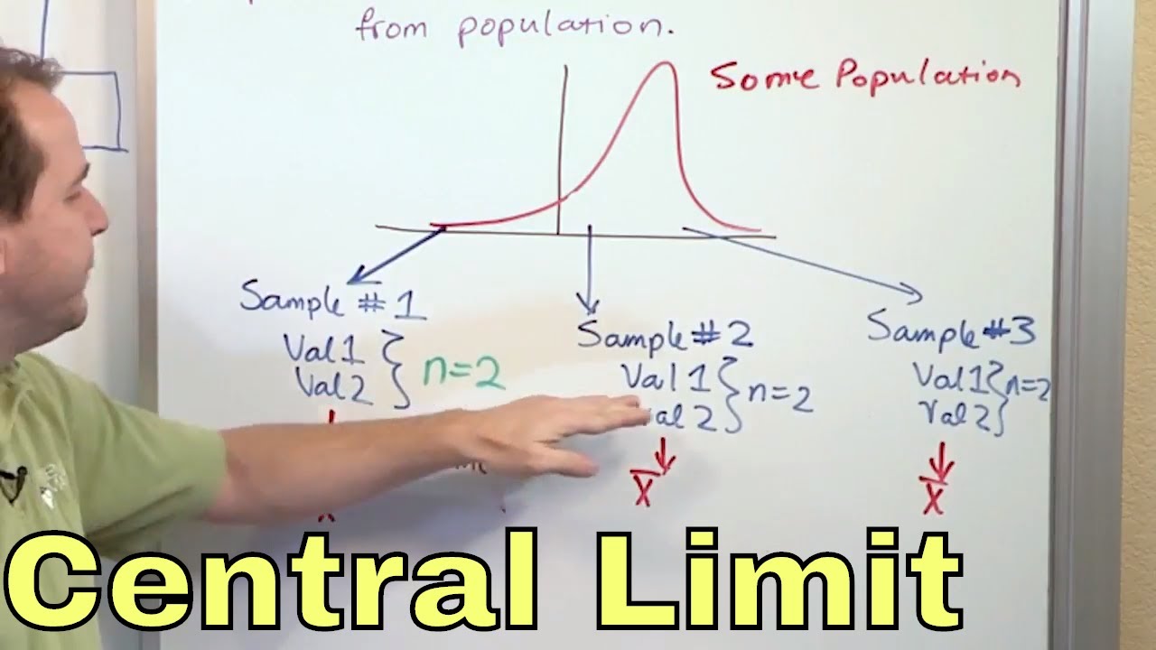
The sampling distribution of sample means is the distribution of all possible sample means from a population.
The mean of the sampling distribution, or the mean of sample means, is denoted as \( \mu_{\bar{x}} \) and is equal to the population mean.
The standard deviation of the sampling distribution, also known as the standard error of the mean (SEM), is denoted as \( \sigma_{\bar{x}} \).
An example using the weights of adult males illustrates the normal distribution of sample means.
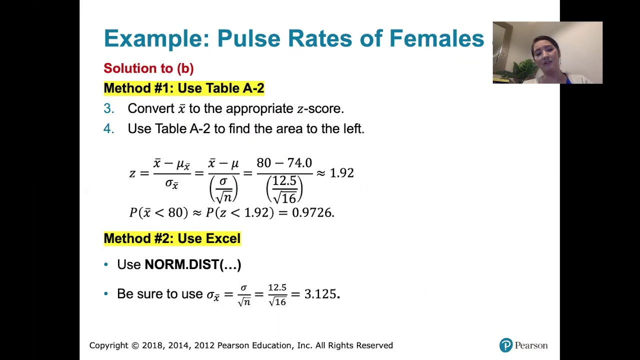
The probability of an individual's weight can be contrasted with the probability of a sample mean exceeding a certain value.
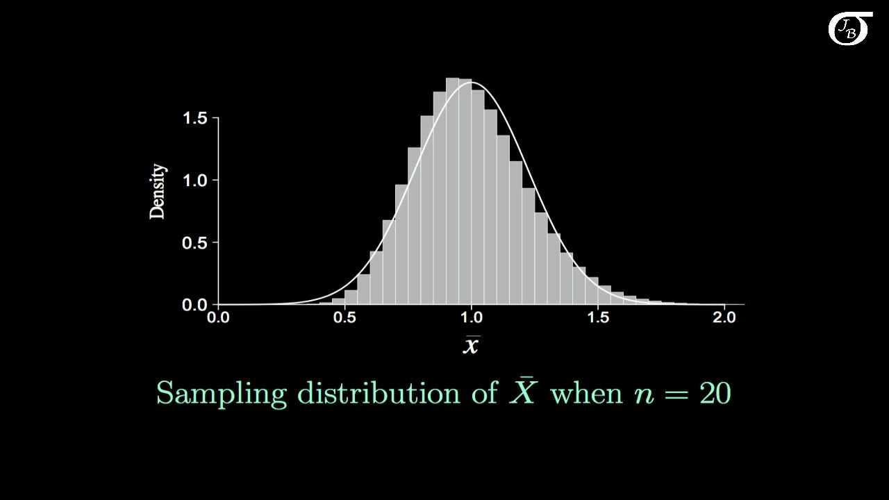
The distribution of sample means becomes more concentrated (taller and skinnier) as the sample size increases.
The central limit theorem clarifies that it is the distribution of sample means, not the sample data, that approaches normality with an increase in sample size.
The theorem does not imply that the original population must be normally distributed for the sample means to form a normal distribution.
The mean and standard deviation of the sample means are closely related to those of the original population in a specific mathematical way.
The central limit theorem is crucial for understanding how sample statistics can be used to make inferences about a population.
The theorem corrects common misconceptions about the distribution of sample data versus sample means.
The standard deviation of the sample means decreases as the square root of the sample size increases, leading to a more precise estimate of the population mean.
The video aims to provide a clear understanding of the central limit theorem's implications for statistical analysis.
Transcripts
Browse More Related Video
02 - What is the Central Limit Theorem in Statistics? - Part 1
6.4.2 The Central Limit Theorem - Probabilities for a Range of Normally Distributed Sample Means
The Central Limit Theorem, Clearly Explained!!!
Introduction to the Central Limit Theorem

Elementary Stats Lesson #13
Z-statistics vs. T-statistics | Inferential statistics | Probability and Statistics | Khan Academy
5.0 / 5 (0 votes)
Thanks for rating: