Riemann sum | MIT 18.01SC Single Variable Calculus, Fall 2010
TLDRIn this recitation, the professor introduces the concept of using Riemann sums to approximate definite integrals, specifically the integral of x cubed from -1 to 3. The lesson involves dividing the interval into four equal subintervals and using left endpoints to estimate the integral's value. The professor visually demonstrates the process by drawing rectangles on a graph, calculating the area of each, and summing them up to find an approximation. The final step includes a formal representation of the Riemann sum and an explanation of the significance of each component in the calculation.
Takeaways
- 👋 The professor introduces the session focused on using Riemann sums to approximate definite integrals.
- 📝 The specific problem given is to use four subintervals and left endpoints to approximate the integral of x cubed from -1 to 3.
- 📊 A rough sketch of y = x cubed is provided to aid in understanding.
- 🕒 The professor gives students time to work on the problem before demonstrating the solution.
- 📐 Four subintervals with left endpoints are used to approximate the integral.
- 📉 The heights of the rectangles are determined by the output at the left endpoint of each subinterval.
- 🔢 The values of y_0, y_1, y_2, and y_3 are calculated based on the function x cubed.
- ➗ The left endpoints are at x = -1, 0, 1, and 2, resulting in y values of -1, 0, 1, and 8 respectively.
- 🟦 The areas of the rectangles are summed to approximate the definite integral, resulting in a total area of 8.
- 🔢 The Riemann sum is written formally as the sum of f(x_i) * delta x from i = 0 to 3.
Q & A
What is the main topic of the recitation session described in the transcript?
-The main topic is using Riemann sums to approximate definite integrals.
What is the function given in the problem to be integrated?
-The function given is f(x) = x^3, or y = x cubed.
Over what interval is the definite integral to be approximated?
-The definite integral is to be approximated over the interval from -1 to 3.
How many subintervals are used to approximate the definite integral in the problem?
-Four subintervals are used for the approximation.
What method of Riemann sums is being used in the approximation?
-The left endpoint method of Riemann sums is being used.
What is the value of delta x in this problem?
-In this problem, delta x is equal to 1, as each subinterval has a unit length.
What are the left endpoints of the subintervals used in the approximation?
-The left endpoints are -1, 0, 1, and 2.
How are the heights of the rectangles determined in the left endpoint method?
-The heights of the rectangles are determined by the function values at the left endpoints of the subintervals.
What is the value of y_0 in the approximation?
-The value of y_0 is the function value at x = -1, which is (-1)^3 or -1.
What is the sum of the areas of the rectangles used to approximate the definite integral?
-The sum of the areas is -1 + 0 + 1 + 8, which equals 8.
How is the Riemann sum represented in the transcript?
-The Riemann sum is represented as the sum from i = 0 to 3 of f(x_i) * delta x.
What is the significance of the negative sign in the area calculation?
-The negative sign indicates that the area below the x-axis is considered as negative when calculating the signed area under the curve.
How can the Riemann sum be written more formally with the x_i values?
-The Riemann sum can be written formally as the sum from i = 0 to 3 of f(x_i), where x_0 = -1, x_1 = 0, x_2 = 1, and x_3 = 2, each multiplied by delta x.
Outlines
📚 Introduction to Riemann Sums for Definite Integrals
The professor begins the recitation by introducing the concept of using Riemann sums to approximate definite integrals. The task is to approximate the integral of the function x^3 from -1 to 3 using four subintervals with left endpoints. The students are given time to work on the problem, which involves sketching the function and understanding the concept of left endpoint rectangles for approximation. The professor also explains the importance of considering the signed area under the curve and how to calculate the area of the rectangles formed by the left endpoints.
📐 Calculating Riemann Sums with Left Endpoints
In this paragraph, the professor demonstrates the calculation of the Riemann sum using the left endpoints of the subintervals. The function f(x) = x^3 is evaluated at the left endpoints x = -1, 0, 1, and 2, yielding values y_0 = -1, y_1 = 0, y_2 = 1, and y_3 = 8. The professor emphasizes the importance of the subscripts representing the interval rather than the x-value. The rectangles' areas are calculated by multiplying the base (delta x, which is 1) by the respective heights (y_values). The sum of these areas, considering the negative area of the first rectangle, results in an approximation of the definite integral. The professor also introduces the formal notation for Riemann sums and how to represent the x-values for each subinterval.
Mindmap
Keywords
💡Riemann sums
💡Definite integral
💡Left endpoints
💡Subintervals
💡Function x^3
💡Signed area
💡Delta x
💡Rectangle heights
💡Output values
💡Sum notation
Highlights
Introduction to using Riemann sums to approximate definite integrals.
Problem statement: Approximate the integral of x^3 from -1 to 3 using 4 subintervals and left endpoints.
Sketch of y = x^3 provided as a starting point.
Explanation of the process to approximate the definite integral using Riemann sums with left endpoints.
Drawing of the 4 subintervals and left endpoints on the graph.
Calculation of the actual value of the estimate using the heights of the rectangles at the left endpoints.
Introduction to different notations for writing Riemann sums.
Demonstration of how to calculate the height of each rectangle using the function's output at the left endpoints.
Evaluation of y_0 to y_3 for the heights of the rectangles.
Explanation of the signed area concept and its application in the approximation.
Calculation of the area of each rectangle and the overall approximation.
Formal representation of the Riemann sum using a summation notation.
Alternative way to write the Riemann sum with designated x values for each subinterval.
Clarification of the subscripts representing intervals rather than x-values.
Final calculation of the Riemann sum approximation: -1 + 1 + 8.
Visual representation of the rectangles and their areas on the graph.
Summary of the process and the result of using Riemann sums to approximate the definite integral of x^3.
Transcripts
Browse More Related Video
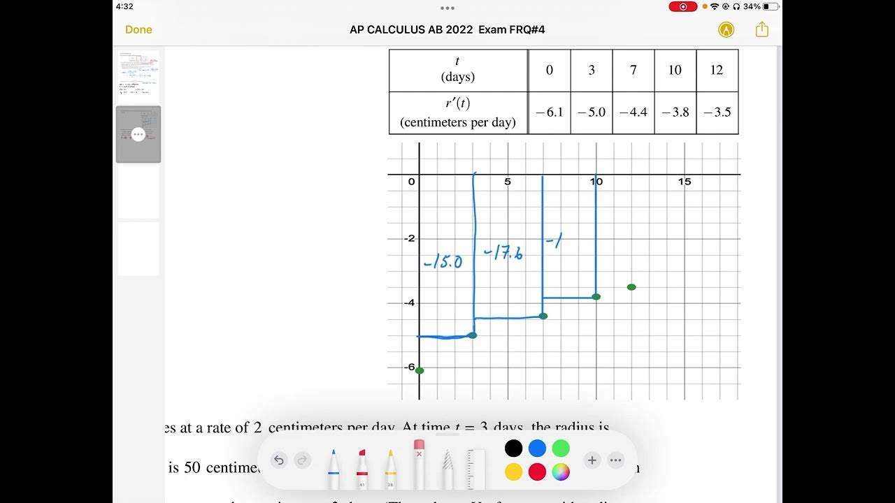
AP CALCULUS AB 2022 Exam Full Solution FRQ#4c
Business Calculus - Math 1329 - Section 5.3 - The Definite Integral and Fundamental Thm of Calculus

Riemann and Trapezoidal Sums from Tables of Values
AP Calculus AB: Lesson 6.2 Part 2 (Limit Definition of Definite Integral)
Left, Right, & Midpoint Riemann Sum Formulas
BusCalc 13.4 Riemann Sums
5.0 / 5 (0 votes)
Thanks for rating: