7.1.4 Estimating a Population Proportion - Margin of Error and Computing Confidence Intervals
TLDRThis video script delves into constructing confidence intervals for estimating a population proportion 'p', emphasizing the margin of error. It explains the sampling distribution of the sample proportion 'p-hat', its properties, and how it's an unbiased estimator of 'p'. The script guides through the process of calculating the margin of error and the confidence interval, highlighting the impact of sample size and confidence level on the error. It concludes with the requirements for constructing a confidence interval and an example of estimating the proportion of inaccurate fast food drive-through orders.
Takeaways
- 📐 The video discusses learning outcome number four from lesson 7.1, focusing on the margin of error and constructing confidence intervals for the population proportion (p).
- 🎯 To construct a confidence interval, the last piece of information needed is the margin of error, which is the maximum likely amount of error in estimating the population proportion.
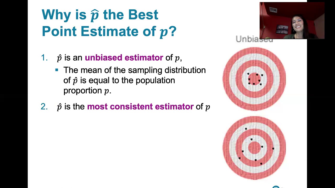
- 📊 The sampling distribution of the sample proportion (p-hat) is normally distributed with a mean equal to the population proportion (p), making it an unbiased estimator.
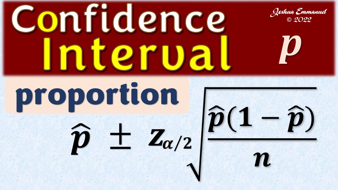
- 🔍 The standard deviation of the sampling distribution of p-hat is approximated using the formula √(p-hat * q-hat / n), where q-hat is 1 - p-hat and n is the sample size.
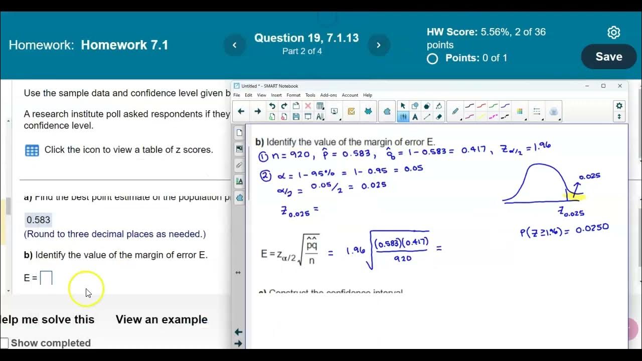
- 📉 The margin of error is calculated using the formula: z * √(p-hat * q-hat / n), where z is the critical z-value corresponding to the desired confidence level.
- 🔢 The confidence interval for p is given by p-hat ± margin of error, indicating the range within which the true population proportion is likely to lie with a certain level of confidence.
- 📈 The confidence level (1 - alpha) determines the width of the confidence interval, with higher confidence levels resulting in wider intervals.
- 🔄 As the sample size (n) increases, the margin of error decreases, leading to a more precise estimate of the population proportion.
- 📝 Three common ways to express a confidence interval are: a compound inequality, a plus-minus format, and interval notation.
- 📚 The video emphasizes the importance of understanding the formulas and their interpretations rather than just memorizing them for tests and quizzes.
- 🔍 Before constructing a confidence interval, it's crucial to check the requirements, such as having a simple random sample and ensuring the conditions for a binomial distribution are met, including at least five successes and five failures.
Q & A
What is the main topic of the video script?
-The main topic of the video script is about constructing confidence intervals for the population proportion 'p', including understanding the margin of error and interpreting confidence intervals.
Why is the sample proportion 'p-hat' considered an unbiased estimator of the population proportion 'p'?
-The sample proportion 'p-hat' is considered an unbiased estimator of the population proportion 'p' because its expected value is equal to the population proportion, meaning it accurately targets the population parameter we want to estimate.
What is the significance of the sampling distribution of 'p-hat' being a normal distribution?
-The significance of the sampling distribution of 'p-hat' being a normal distribution is that it allows us to associate it with a standard normal distribution through certain conversions, which is useful for constructing confidence intervals.
What is the margin of error and how is it used in constructing a confidence interval?
-The margin of error is the maximum likely amount of error between the estimate (sample proportion 'p-hat') and the population proportion 'p'. It is used in constructing a confidence interval by adding and subtracting it from the sample proportion to find the range within which the true population proportion is likely to fall.
How is the standard deviation of the sampling distribution of 'p-hat' approximated?
-The standard deviation of the sampling distribution of 'p-hat' is approximated using the formula sqrt(p-hat * q-hat / n), where p-hat is the sample proportion, q-hat is one minus p-hat, and n is the sample size.
What is the relationship between the confidence level and the margin of error?
-The confidence level determines the range of values within which we expect the true population proportion to fall. A higher confidence level results in a larger margin of error to ensure a wider range of values is captured, thus increasing the certainty of the estimate.
What are the conditions that need to be met before constructing a confidence interval for a population proportion?
-Before constructing a confidence interval for a population proportion, we need to ensure that we have a simple random sample, the conditions for a binomial distribution are met (fixed number of trials, independence of trials, two possible outcomes, constant probabilities, and at least five successes and five failures), and that the normal distribution is a suitable approximation for the binomial distribution.
How does the sample size affect the margin of error?
-As the sample size increases, the margin of error decreases. This is because a larger sample size provides a better representation of the population, leading to a more precise estimate with less potential error.
What are the three different ways to represent a confidence interval for a population proportion 'p'?
-The three different ways to represent a confidence interval for a population proportion 'p' are: 1) stating the range of values we expect the true population proportion to lie in, 2) stating the point estimate with the margin of error as plus or minus, and 3) using interval notation to express the same information.
Can you provide an example from the script where a confidence interval is constructed for a population proportion?
-Yes, an example from the script is constructing a 95% confidence interval for the portion of fast food drive-through orders that are inaccurate at McDonald's, based on a study where there were 33 inaccurate orders out of 362 orders.
Outlines
📊 Introduction to Margin of Error and Confidence Intervals
This paragraph introduces the concept of the margin of error and confidence intervals for estimating a population proportion, denoted as 'p'. It explains that the sample proportion, 'p-hat', is an unbiased estimator of 'p', meaning its expected value is equal to the population proportion. The paragraph also discusses the normal distribution of the sampling distribution of 'p-hat' and how it can be converted to a standard normal distribution for easier analysis. The margin of error is introduced as the difference between the mean of the sampling distribution and the upper bound indicated by a critical value, which is part of constructing a confidence interval.
🔍 Understanding Confidence Intervals and Margin of Error
The second paragraph delves deeper into the concept of confidence intervals, explaining how they provide an estimated range for the true population proportion 'p'. It discusses the relationship between the sample proportion 'p-hat', the margin of error 'e', and the confidence level (1 - alpha). The paragraph illustrates how to rearrange the inequality to express 'p' in terms of 'p-hat' and the margin of error, thus forming the confidence interval. It emphasizes that the margin of error represents the maximum likely amount of error in the estimate and is calculated using a specific formula involving the critical z-value and the standard deviation of 'p-hat'.
📐 The Formula for Margin of Error and Its Components
This paragraph focuses on the formula for calculating the margin of error, which is essential for determining the confidence interval. It explains that the margin of error is the maximum likely amount of error between the sample proportion 'p-hat' and the true population proportion 'p'. The formula involves the critical z-value for the given confidence level, the standard deviation of 'p-hat', and the sample size 'n'. The paragraph also discusses how the margin of error changes with different confidence levels and sample sizes, noting that a larger sample size typically results in a smaller margin of error.
📉 The Impact of Sample Size and Confidence Level on Margin of Error
The fourth paragraph explores the relationship between sample size, confidence level, and the margin of error. It explains that as the sample size increases, the margin of error decreases, which makes intuitive sense because a larger sample is more representative of the population. Conversely, as the confidence level increases, the margin of error increases because a higher level of certainty requires a wider interval to capture the true population proportion. The paragraph reinforces the importance of understanding these relationships when constructing and interpreting confidence intervals.
📝 Steps to Compute and Interpret Confidence Intervals
The final paragraph outlines the steps to compute and interpret confidence intervals for a population proportion. It emphasizes the importance of checking the requirements for a valid analysis, such as having a simple random sample and meeting the conditions for a binomial distribution. The paragraph then details the process of identifying known values like 'p-hat', 'q-hat', the confidence level, and sample size 'n', followed by computing the critical value and the margin of error. Finally, it describes how to calculate the upper and lower limits of the confidence interval and presents different ways to express the interval, including a range, point estimate with error, and interval notation.
🏗️ Applying Confidence Intervals: A Practical Example
This paragraph presents a practical example of applying the concepts of confidence intervals to real-world data. It uses the data from a study on the accuracy of fast food drive-through orders at McDonald's, where 33 out of 362 orders were inaccurate. The paragraph guides through the process of constructing a 95% confidence interval for the proportion of inaccurate orders, demonstrating how to put the theoretical concepts into practice.
Mindmap
Keywords
💡Margin of Error
💡Confidence Interval
💡Population Proportion (p)
💡Sample Proportion (p-hat)
💡Sampling Distribution
💡Normal Distribution
💡Unbiased Estimator
💡Confidence Level
💡Critical Value
💡Binomial Distribution
Highlights
The video discusses learning outcome number four from lesson 7.1 about margin of error and constructing confidence intervals for the population proportion p.
Almost all necessary information for constructing a confidence interval is covered except for the margin of error, which is the focus of the discussion.
The sampling distribution of the sample proportion p-hat is normally distributed with a mean equal to the population proportion p, making it an unbiased estimator.
The standard deviation of the sampling distribution of p-hat is approximated using the formula √(p-hat * q-hat / n).
Margin of error is the maximum likely amount of error and is calculated using a specific formula involving the critical z-value and the standard deviation approximation.
A confidence interval provides an estimated range for the true population proportion with a certain level of confidence.
The confidence interval is computed by adding and subtracting the margin of error from the sample proportion p-hat.
The video emphasizes the importance of understanding why formulas are used and how to interpret them correctly.
As sample size increases, the margin of error decreases, leading to more precise estimates of the population proportion.
Higher confidence levels result in wider confidence intervals and larger margins of error.
The video explains the conditions required for constructing a confidence interval, including having a simple random sample and meeting binomial distribution conditions.
At least five successes and five failures are needed to ensure a normal distribution is a suitable approximation for the binomial distribution.
The process of constructing a confidence interval involves identifying known values, computing the critical value, margin of error, and the interval limits.
Three different formats are presented for representing a confidence interval for a population proportion.
An example is provided to demonstrate the computation of a 95% confidence interval for the proportion of inaccurate fast food drive-through orders.
The video concludes by stressing the importance of understanding the concepts behind the formulas rather than just memorizing them for tests and quizzes.
Transcripts
Browse More Related Video
7.1.1 Estimating a Population Proportion - The Best Point Estimate, Our Sample Proportion p-Hat
Confidence Interval for a population proportion | Solved Problems

Elementary Stats Lesson #15
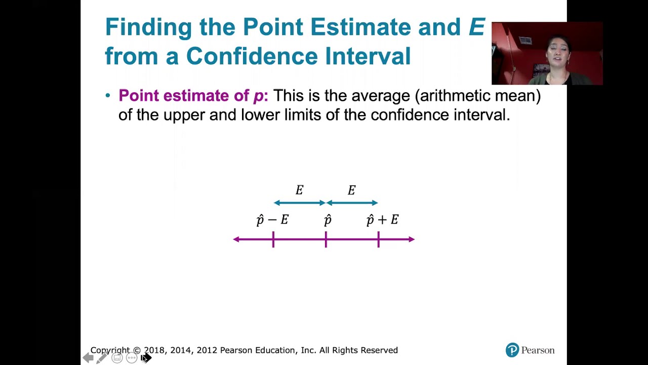
7.1.5 Estimating a Population Proportion - Given a Confidence Interval, Find p Hat and E.
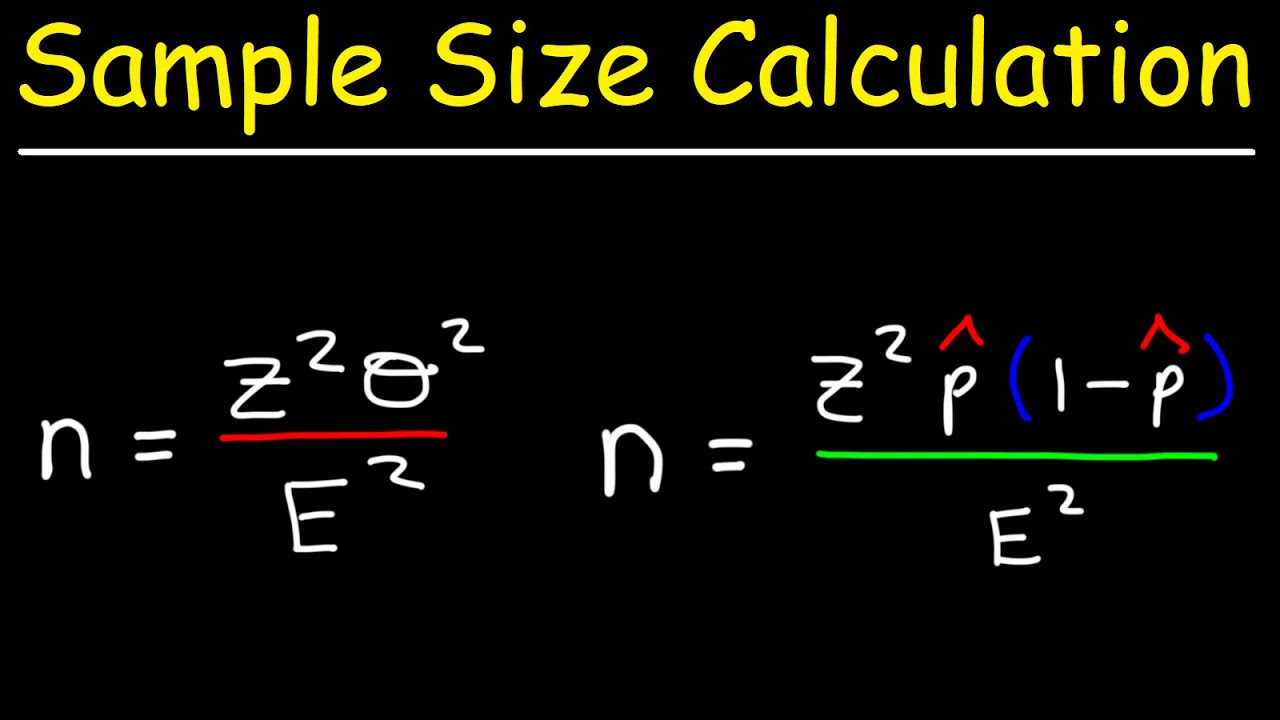
How To Calculate The Sample Size Given The Confidence Level & Margin of Error
Math 14 7.1.13 Find the point estimate, margin of error & confidence interval of pop. proportion p.
5.0 / 5 (0 votes)
Thanks for rating: