Hypothesis Testing - Difference of Two Means - Student's -Distribution & Normal Distribution
TLDRThis educational video delves into hypothesis testing for two sample means through detailed examples. The first scenario compares the final exam scores of students from two classes to assess the performance difference between two teachers, using a t-distribution due to small sample sizes. The second example investigates whether a new oil refinery factory significantly outperforms an old one, employing a z-test for larger sample sizes. Through step-by-step calculations, critical values, and hypothesis formulation, the video demonstrates how to reject or fail to reject the null hypothesis, providing clear insights into statistical testing at different significance levels.
Takeaways
- 📚 The video covers hypothesis testing with two sample means to determine significant differences in performance or measurements.
- 📝 For the first example, the comparison is between the final exam scores of students from two different classes to evaluate the performance of two teachers.
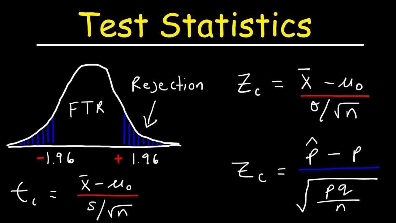
- 🏆 The null hypothesis (H0) posits no difference in means (mu1 = mu2), while the alternative hypothesis (H1) suggests a significant difference (mu1 != mu2).
- 📈 The significance level (alpha) is set at 5% for the first example, indicating a 95% confidence level in the results.
- ✏️ T-distribution is chosen for analysis due to the small sample sizes (n1=15, n2=12), as per the threshold of n<30 for using T over normal distribution.
- 🔢 Degrees of freedom are calculated using a specific formula to find the critical t-values for hypothesis testing.
- 📗 The calculated t-value is compared against the critical t-value to decide on rejecting or accepting the null hypothesis.
- ✔️ The conclusion for the first example is that there is a significant difference in teacher performance, as the calculated t-value falls into the rejection region.
- 📊 The second example explores the efficiency of two factories, with a 10% significance level indicating a 90% confidence level.
- ⚡ The Z-test is used for the second example due to larger sample sizes (n1=40, n2=36), which justifies using the normal distribution.
- 🛠 Conclusion for the second example indicates a significant difference between the two factories' efficiencies, as the calculated z-value also falls into the rejection region.
Q & A
What statistical test is used to compare the performance of two teachers based on student scores?
-A t-test for independent samples is used to compare the performance.
What are the null and alternative hypotheses for the test comparing two teachers' performances?
-The null hypothesis is that the mean scores for both classes are equal (mu1 - mu2 = 0), and the alternative hypothesis is that the mean scores are not equal (mu1 - mu2 ≠ 0).
Why is a t-distribution used instead of a normal distribution for the test comparing two teachers?
-A t-distribution is used because the sample sizes are small (less than 30), which is appropriate for estimating the population mean when the sample size is small and the population standard deviation is unknown.
How are degrees of freedom calculated for the t-test comparing the two classes?
-Degrees of freedom are calculated using a specific formula that accounts for the sample sizes and standard deviations of both groups, resulting in a value that is rounded to the nearest whole number.
What indicates a significant difference between the two teachers' performances at the 5% significance level?
-A significant difference is indicated if the calculated t-value falls within the rejection region, leading to the rejection of the null hypothesis.
What statistical test is used to compare the refining rates of two factories?
-A z-test is used to compare the refining rates of the two factories, as the sample sizes are large (greater than 30).
What are the null and alternative hypotheses for comparing the refining rates of the old and new factories?
-The null hypothesis is that the refining rates of both factories are the same, and the alternative hypothesis is that the rates are different.
Why is the z-test chosen over the t-test for comparing the refining rates of two factories?
-The z-test is chosen because both sample sizes are greater than 30, which allows for the use of the normal distribution assumption in large samples.
What does the rejection of the null hypothesis imply about the refining rates of the old and new factories?
-Rejecting the null hypothesis implies that there is a statistically significant difference between the refining rates of the old and new factories.
What significance level and confidence level are used when comparing the refining rates of the two factories?
-A 10% significance level (alpha = 0.10) and a 90% confidence level are used for the comparison.
Outlines
📊 Hypothesis Testing with Two Sample Means
This segment introduces a hypothesis test comparing the final exam scores of students from two different classes to assess the teaching performance differences. With a sample from each class (15 and 12 students respectively), mean scores and standard deviations are provided for both. The task is to determine if there's a significant difference at the 5% significance level between the two teachers' performances. The process involves outlining sample sizes, means, standard deviations, setting up null and alternative hypotheses, and deciding on the distribution type (t-distribution due to small sample sizes) to use for further analysis.
🔍 Calculating Degrees of Freedom and Critical T-Values
The focus shifts to calculating the degrees of freedom using a detailed formula that takes into account the sample sizes, standard deviations, and a step-by-step calculation is illustrated. The degrees of freedom are rounded to the nearest whole number to determine the critical t-value from a t-distribution table. This step is crucial for establishing the boundaries (rejection regions) within which the hypothesis test will be evaluated. The critical t-value is identified based on the degrees of freedom and the significance level.
📐 Determining the Calculated T-Value
This part explains how to calculate the t-value using the sample data. The formula involves the difference in sample means, standard deviations, and sample sizes. A specific calculated t-value is derived and compared against the critical t-value to decide on rejecting or not rejecting the null hypothesis. The conclusion is drawn that there is a significant difference in teacher performances, as indicated by the calculated t-value falling within the rejection region.
🏭 Analysis of Two Factories' Production Rates
The script transitions to a second example problem involving a business decision about investing in a new oil refinery factory. Sample sizes, mean rates of oil production, and standard deviations for both an old and a new factory are provided. The task is to evaluate if there's a significant difference at the 10% significance level between the two factories' production rates. After setting up hypotheses, the segment discusses choosing between a z-test and a t-test based on the sample sizes, eventually opting for the z-test due to large sample sizes.
Mindmap
Keywords
💡Hypothesis Tests
💡Significance Level
💡Null Hypothesis
💡Alternative Hypothesis
💡Sample Mean
💡Standard Deviation
💡T Distribution
💡Degrees of Freedom
💡Critical Value
💡Rejection Region
Highlights
A hypothesis test was conducted to compare the performance of two teachers using students' final exam scores.
The first class had a sample size of 15 students with a mean score of 82 and a standard deviation of 2.4.
The second class had a sample size of 12 students with a mean score of 84 and a standard deviation of 1.7.
The test aimed to identify any significant difference in teacher performance at the 5 percent significance level.
The null hypothesis assumed no difference in mean performance between the two classes.
A t-distribution was chosen for analysis due to the small sample sizes (less than 30).
The degrees of freedom for the test were calculated using a specific formula and rounded to the nearest whole number, resulting in 25 degrees of freedom.
The critical t-value was determined from the t-distribution table based on the degrees of freedom and the alpha level.
The calculated t-value was found to fall in the rejection region, leading to the rejection of the null hypothesis.
The conclusion was that there is a significant difference in the performance of the two teachers.
A second hypothesis test was proposed to compare the efficiency of two factories in refining oil.
The old factory had a sample size of 40 with a mean refining rate of 3.1 liters per second.
The new factory had a sample size of 36 with a mean refining rate of 3.8 liters per second.
The test aimed to identify any significant difference in refining efficiency at the 10 percent significance level.
The z-test was used for analysis due to the large sample sizes (greater than 30).
The calculated z-value indicated a significant difference, leading to the rejection of the null hypothesis and confirming the new factory's higher efficiency.
Transcripts
Browse More Related Video
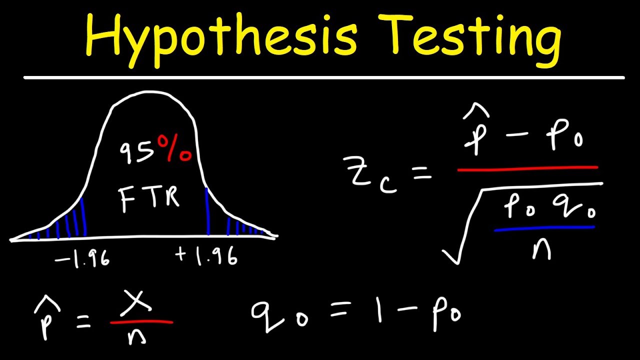
Hypothesis Testing - Solving Problems With Proportions
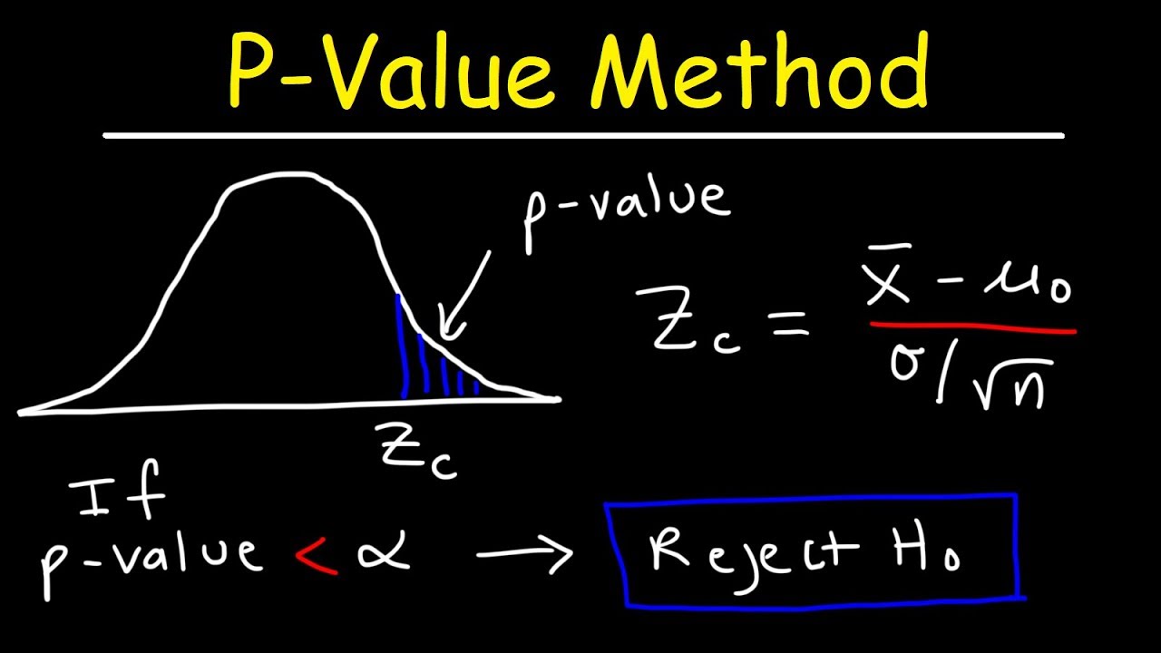
P-Value Method For Hypothesis Testing
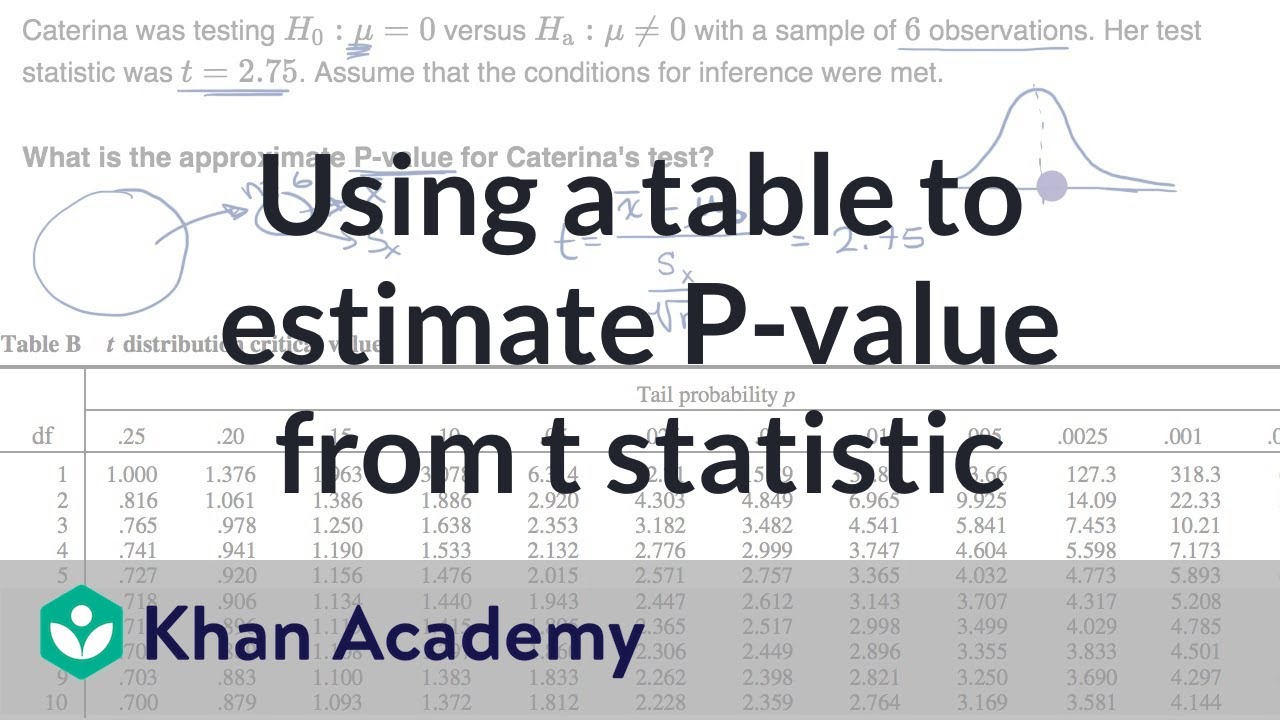
Using a table to estimate P-value from t statistic | AP Statistics | Khan Academy
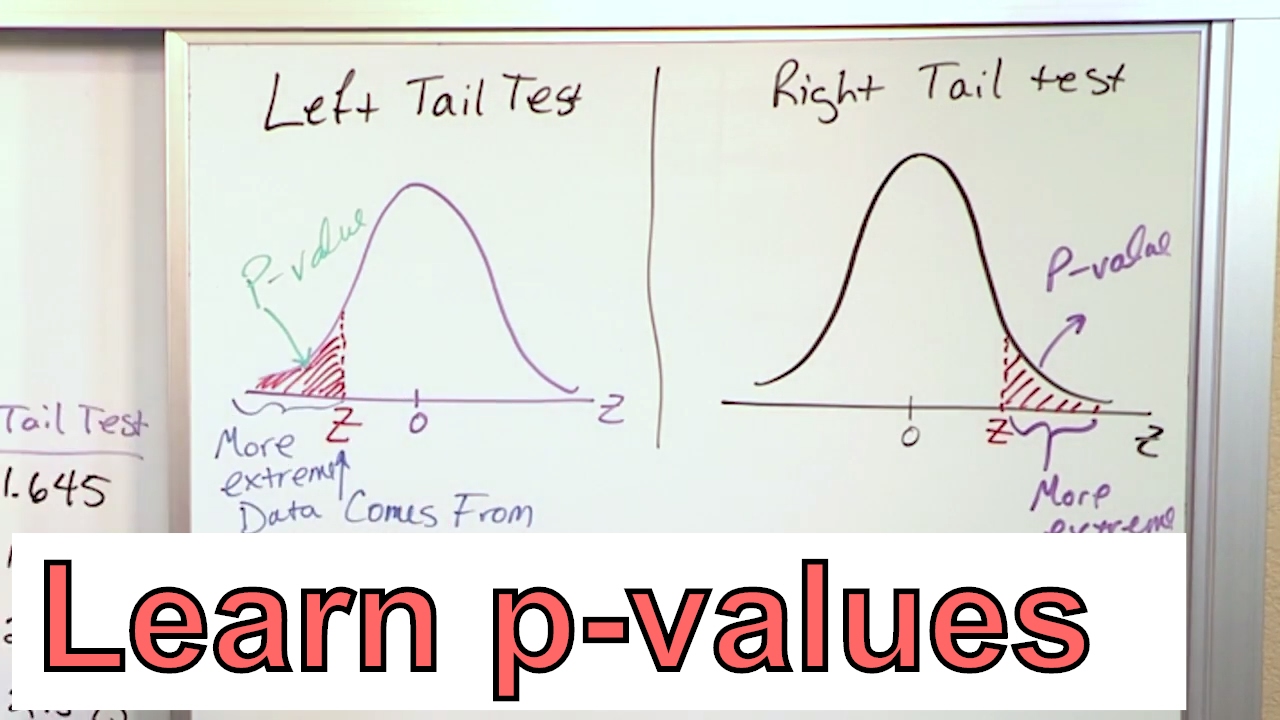
Calculate the P-Value in Statistics - Formula to Find the P-Value in Hypothesis Testing
Test Statistic For Means and Population Proportions

Explaining The One-Sample t-Test
5.0 / 5 (0 votes)
Thanks for rating: