2022 AP Calculus AB Exam FRQ #5
TLDRThis video tutorial covers problem number five from the 2022 Calc AB exam, focusing on a differential equation. The presenter begins by sketching a solution curve on a slope field, using the point (1,2) as a starting reference. They then calculate the slope at this point and use it to write an equation for the tangent line, which helps approximate the function value at another point, 0.8. The concavity of the function is discussed to determine if the approximation is an overestimate or underestimate. The video concludes with solving the differential equation using the method of separation of variables, offering detailed step-by-step guidance.
Takeaways
- 📚 The video discusses solving a differential equation problem from the 2022 Calc AB exam.
- 🔍 The differential equation given is ( dy/dx = 1/2 sin(pi/2x) sqrt(y + 7) ).
- 📈 A particular solution y = f(x) is sought with the initial condition f(1) = 2.
- 🌊 The slope field for the differential equation is visualized as flowing water to sketch the solution curve.
- 📶 The function f is suggested to be an even function due to the symmetry observed in the slope field.
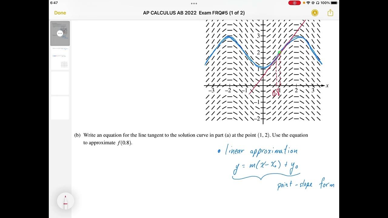
- 🆗 Part A involves sketching the solution curve through the point (1,2).
- 🔢 For Part B, the slope of the tangent line at the point (1,2) is calculated using the given differential equation.
- 🔍 The slope is found to be 3/2 by substituting x = 1 and y = 2 into the equation.
- 🔑 Using the tangent line equation, an approximation for f(0.8) is made, which is approximately 1.7.
- ⏏️ It is determined that the approximation for f(0.8) is an underestimate because f''(x) > 0 for x between -1 and 1, indicating the function is concave up.
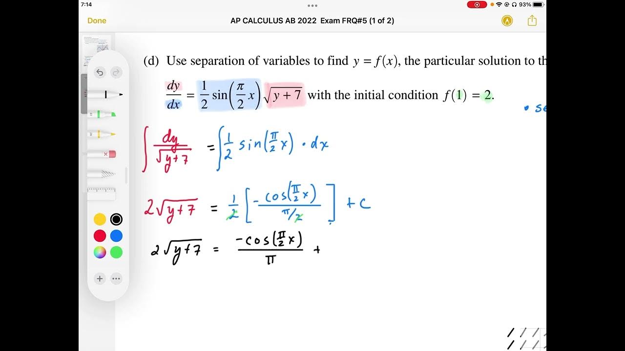
- 🧩 The method of separation of variables is used in Part C to find the particular solution to the differential equation.
- 🧮 Integration is performed on both sides of the separated equation, and the constant of integration c is solved using the initial condition.
- 🎯 The final particular solution y = f(x) is obtained after methodically solving for y.
Q & A
What is the differential equation problem discussed in the video?
-The video discusses a differential equation problem from the 2022 Calc AB exam. The equation is given by dy/dx = (1/2) * sin(π/2 * x) * sqrt(y + 7).
What is the initial condition for the particular solution y = f(x)?
-The initial condition for the particular solution y = f(x) is that f(1) = 2.
How does the video describe the process of sketching the solution curve?
-The video suggests visualizing the slope field as if it were flowing water. One would jump into the water at the given point and follow the contours to sketch the solution curve.
What is the significance of the function f being an even function?
-The significance of f being an even function is that it is symmetric about the y-axis, which is suggested by the slope field's contours.
How is the slope of the tangent line to the solution curve at the point (1, 2) determined?
-The slope is determined by evaluating dy/dx at the point (1, 2), which involves substituting x with 1 and y with 2 in the given differential equation.
What is the equation of the tangent line to the solution curve at the point (1, 2)?
-The equation of the tangent line is y - 2 = (3/2) * (x - 1).
How is the approximation for f(0.8) obtained?
-The approximation for f(0.8) is obtained by plugging x = 0.8 into the equation of the tangent line and solving for y.
What is the implication of f''(x) > 0 for x between -1 and 1?
-The implication of f''(x) > 0 for x between -1 and 1 is that the function f(x) is concave up on this interval.
Why is the approximation for f(0.8) considered an underestimate?
-Since f(x) is concave up on the interval from -1 to 1, the tangent line lies below the curve, which means the approximation for f(0.8) is an underestimate.
What method is used to find the particular solution to the differential equation?
-The method used to find the particular solution is separation of variables.
How is the constant of integration, c, determined in the solution?
-The constant of integration, c, is determined by using the initial condition f(1) = 2 and solving for c in the integrated equation.
What is the final form of the particular solution y = f(x)?
-The final form of the particular solution y = f(x) is obtained after solving for y from the integrated equation, which involves squaring both sides and then isolating y.
Outlines
📚 Introduction to Differential Equation Problem
The video begins with an introduction to a differential equation problem from the 2022 Calculus AB exam. The problem involves a straightforward differential equation, and the presenter outlines the steps to find a particular solution, y = f(x), with the initial condition f(1) = 2. The function f is defined for all real numbers. The presenter also discusses sketching the solution curve through the point (1,2) by visualizing the slope field as flowing water and identifying relative maxima and minima.
📐 Sketching the Solution Curve and Tangent Line Approximation
The presenter explains how to sketch the solution curve for the differential equation, emphasizing the shape of the curve in relation to the slope field. The video then moves on to finding the equation of the tangent line to the solution curve at the point (1,2). By evaluating the derivative of y with respect to x at this point, the slope of the tangent line is determined. Using the point-slope form, the equation of the tangent line is established. The presenter then approximates the value of f(0.8) using the tangent line and discusses a potential issue with the approximation.
🔍 Analysis of the Tangent Line Approximation
The video continues with an analysis of whether the approximation found for f(0.8) in the previous section is an overestimate or an underestimate. Given that the second derivative of f is greater than zero for x between -1 and 1, indicating that the function is concave up, the presenter concludes that the tangent line is below the curve, leading to an underestimate of f(0.8).
🧮 Solving the Differential Equation Using Separation of Variables
The presenter then tackles the main part of the problem by using the method of separation of variables to find the particular solution to the given differential equation. The process involves isolating y in the equation and integrating both sides. Through a series of algebraic manipulations and substitutions, including recognizing a missing factor of (pi/2) in the integral, the presenter integrates the right side of the equation and solves for the constant of integration using the initial condition. The final step involves solving for y to express it as a function of x, providing the particular solution to the differential equation.
Mindmap
Keywords
💡Differential Equation
💡Slope Field
💡Particular Solution
💡Initial Condition
💡Tangent Line
💡Approximation
💡Concavity
💡Separation of Variables
💡Integration
💡Implicit Differentiation
💡Product Rule
Highlights
The video discusses solving a differential equation problem from the 2022 Calc AB exam, emphasizing its straightforward nature.
The differential equation is dy/dx = (1/2) * sin(π/2x) * sqrt(y) + 7, with a particular solution y = f(x).
The initial condition given is f(1) = 2, with the function f defined for all real numbers.
Part A involves sketching the solution curve through the point (1, 2), using the concept of a slope field.
The slope field is visualized as flowing water, with the solution curve following the contours.
The function f is suggested to be an even function based on the slope field's characteristics.
Part B requires writing an equation for the line tangent to the solution curve at the point (1, 2).
The slope is found by evaluating dy/dx at the point (1, 2), using substitution.
The tangent line equation is derived, and used to approximate f(0.8) ≈ 1.7.
It is known that f''(x) > 0 for x between -1 and 1, which indicates the function is concave up.
The approximation found in Part B for f(0.8) is identified as an underestimate due to the concavity.
Separation of variables is used in Part C to find the particular solution to the differential equation.
The integration process involves rewriting the left-hand side and applying u-substitution to the right-hand side.
The constant of integration, c, is solved using the initial condition f(1) = 2.
The final step involves solving for y to express y as a function of x, providing the particular solution.
The process is broken down into meticulous steps to avoid errors in solving for y.
The video concludes with the derived differential equation solution, y = f(x), and wishes viewers good luck.
Transcripts
Browse More Related Video


5.0 / 5 (0 votes)
Thanks for rating: